Collaborating Filtering for Mere Mortals Part 2: A Neural Network Approach
Introduction
In my previous post, I wrote about how matrix based collaborative filtering works and went through a simple example implementation using the Surprise package in python. Continuing on with that topic, I wanted to explore an alternative approach to this problem that uses neural networks.
Recall that our previous approach was essentially about creating a matrix that maps users and items. This matrix is made up of previously known ratings from users. In our example, the items were movies and the ratings were scores from 0.5 to 5.0. Since not all users have watched all movies, the matrix in question is very sparse. The goal, then, is to attempt to find a solution that fills in the gaps.
Using matrix factorization and singular value decomposition is just one approach to solving this problem. Another approach involves using neural networks, or more accurately multi-layer perceptrons or “MLPs”.
The MovieLens Dataset
To demonstrate how this works, I am again using the MovieLens 100k dataset that consists of users, movies and rankings. More information about the MovieLens dataset can be found on the GroupLens website.
Network Structure
Neural networks similar to the one in this example are frequently referred to as “deep learning”, but IMO it really is not. As we will see below, the network in use here has only a few layers. Deep learning networks typically have dozens or more layers and lots of parameters. For example, Yolo V8 has 53 convolutional layers alone, and GPT3.5 has 96 layers and 175B trainable parameters. These types of networks are DEEP! As we will see, the neural network in this example is very basic and very shallow.
To understand how the network is structured, let’s start with a simple diagram. The following diagram was created from the torchviz packaged. We can see that the network starts with two main sets of inputs, user_factors and item_factors.
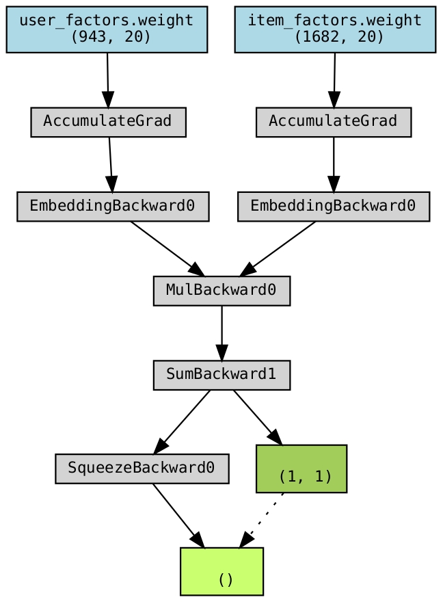
The key thing to understand here is that an initial “embedding” is taking place in order to feed information into the network. This is done by creating a mapping from a given user and an embedding vector of some length. In the case of my code for the movie example, the embedding vectors have a length of 20. Initially, the values of the embedding vectors are randomized. As the network continues to train, back propagation is used to update these values. As training progresses, the embedding vectors start to “understand the latent structure” hidden in the data.
As with the previous example with collaborative filtering, the neural network approach also suffers from the “cold-start problem.” The cold-start problem refers to the difficult of providing accurate recommendations for new or “cold” users that have limited historical data. (Yes, I did lift that from ChatGPT.) Simply put, in order for us to do inference, we are going to have to have trained our model on at least some information for a given user and item.
Introducing Factor Biases
One of the challenges in building models like this is that users and items can suffer from biases. For example, one user might be particularly generous in their rankings compared to others. Or, certain items may have been reviewed more times than others. In the paper “Factorization Meets the Neighborhood: a Multifaceted Collaborative Filtering Model.” (Proceedings of the 14th ACM SIGKDD international conference on Knowledge discovery and data mining (KDD ‘08), pp. 426-434. DOI: 10.1145/1401890.1401944), author Yehuda Koren presents a way to deal with this situation by introducing a vector for user and item biases. The addition of these bias vectors can be seen in the next diagram.
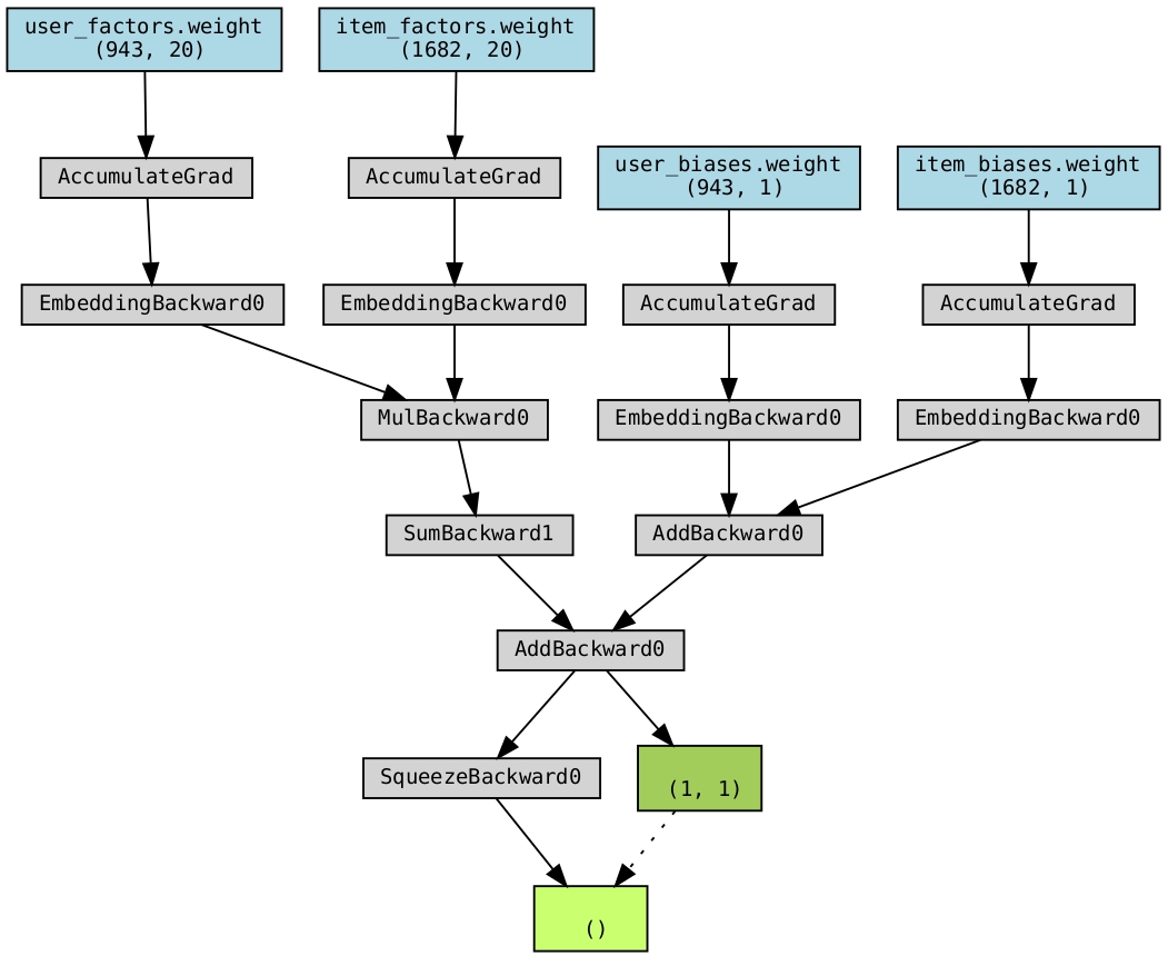
Note that the bias vectors are of length 1. They are basically a trained value that boosts or discounts the overall value of the prediction for a given user and item. Like the embedding vectors, these values are updated as the network gets trained.
Some Code
The following includes some code that will train a neural network to make ratings predictions based on the MovieLens 100k dataset. In this code, I have configured the system to run 450 training epochs. With my Quadro GP100 (which is a slightly older GPU), this process took about an hour.
import os
import pandas as pd
import torch
import torch.nn as nn
import torch.optim as optim
from torch.utils.data import Dataset, DataLoader, random_split
from torchviz import make_dot
import logging

# Set up logging
logging.basicConfig(level=logging.DEBUG)

# Set the device (CPU/GPU)
device = torch.device("cpu")
if torch.cuda.is_available():
    device = torch.device("cuda")
    print(f"PyTorch is using GPU: {torch.cuda.get_device_name(0)}")
else:
    print("PyTorch is using CPU")

# Define a custom dataset class for MovieLens data
class MovieLensDataset(Dataset):
    def __init__(self, data_path):
        # Load data from a CSV file into a Pandas DataFrame
        self.data = pd.read_csv(os.path.join(data_path, "u.data"), sep="\t", header=None, names=["user_id", "item_id", "rating", "timestamp"])

    def __len__(self):
        return len(self.data)

    def __getitem__(self, idx):
        return self.data.iloc[idx]

# Define a recommender system model using PyTorch nn.Module
class RecommenderSystem(nn.Module):
    def __init__(self, n_users, n_items, n_factors=20):
        super().__init__()
        # Embedding layers for user and item factors
        self.user_factors = nn.Embedding(n_users, n_factors)
        self.item_factors = nn.Embedding(n_items, n_factors)
        # Embedding layers for user and item biases
        self.user_biases = nn.Embedding(n_users, 1)
        self.item_biases = nn.Embedding(n_items, 1)

    def forward(self, user, item):
        # Perform forward pass through the model
        user_factors = self.user_factors(user)
        item_factors = self.item_factors(item)
        user_biases = self.user_biases(user)
        item_biases = self.item_biases(item)

        rating = (user_factors * item_factors).sum(dim=1, keepdim=True)
        rating += user_biases + item_biases
        return rating.squeeze()

    def visualize_network(self, user, item):
        rating = self.forward(user, item)
        dot = make_dot(rating, params=dict(self.named_parameters()))
        return dot

# Method for training the model for one epoch
def train_epoch(model, train_loader, criterion, optimizer, device):
    model.train()
    for i in range(1, len(train_loader) + 1):
        row = train_loader.dataset.dataset.data.iloc[i - 1]
        try:
            user = torch.LongTensor([row["user_id"]])
            item = torch.LongTensor([row["item_id"]])
            rating = torch.FloatTensor([row["rating"]])

            user, item, rating = user.to(device), item.to(device), rating.to(device)

            optimizer.zero_grad()
            pred = model(user, item)
            loss = criterion(pred, rating.squeeze().float())
            loss.backward()
            optimizer.step()
        except Exception as e:
            print("Something blew up in training on row #{}!".format(i))
            print("Row: {}".format(row))
            exit(1)

# Method for evaluating the model
def evaluate(model, test_loader, device):
    model.eval()
    total_loss = 0
    total_count = 0

    with torch.no_grad():
        for i in range(1, len(test_loader) + 1):
            try:
                row = test_loader.dataset.dataset.data.iloc[i - 1]
                user = torch.LongTensor([row["user_id"]])
                item = torch.LongTensor([row["item_id"]])
                rating = torch.FloatTensor([row["rating"]])

                user, item, rating = user.to(device), item.to(device), rating.to(device)
                pred = model(user, item)
                total_loss += ((pred - rating) ** 2).sum().item()
                total_count += 1 #pred.size(0)
            except Exception as e:
                print("Something blew up in testing on row #{}!".format(i))
                print("Row: {}".format(row))
                exit(1)

    return total_loss / total_count

# Method to display predictions
def display_predictions(model, test_loader, item_names, device):
    model.eval()
    with torch.no_grad():
        for i in range(1, 10):
            row = test_loader.dataset.dataset.data.iloc[i - 1]
            user = torch.LongTensor([row["user_id"]])
            item = torch.LongTensor([row["item_id"]])
            rating = torch.FloatTensor([row["rating"]])

            user, item, rating = user.to(device), item.to(device), rating.to(device)
            pred = model(user, item)
            item_name = item_names.loc[item_names['item_id'] == row["item_id"], 'title'].values[0]
            print(f"Item Name: {item_name}, Actual Value: {rating.item()}, Predicted Value: {pred.item()}")

def get_item(loader, n):
    row = loader.dataset.dataset.data.iloc[n]
    user = torch.LongTensor([row["user_id"]])
    item = torch.LongTensor([row["item_id"]])
    rating = torch.FloatTensor([row["rating"]])
    return user.to(device), item.to(device), rating.to(device)

# Main function
def main():

    data_path = "./data/ml-100k"
    # Initialize MovieLens dataset and item names
    dataset = MovieLensDataset(data_path)
    item_names = pd.read_csv(os.path.join(data_path, "u.item"), sep="|", encoding="latin-1", header=None, names=["item_id", "title"], usecols=[0, 1])

    # Get the number of unique users and items
    n_users = dataset.data["user_id"].nunique()
    n_items = dataset.data["item_id"].nunique()

    # Split dataset into training and test sets
    train_size = int(0.9 * len(dataset))
    test_size = len(dataset) - train_size
    train_dataset, test_dataset = random_split(dataset, [train_size, test_size])

    # Create data loaders for training and testing
    train_loader = DataLoader(train_dataset, batch_size=32, shuffle=True)
    test_loader = DataLoader(test_dataset, batch_size=1, shuffle=False)


    # Initialize the recommender system model, criterion, and optimizer
    model = RecommenderSystem(n_users, n_items).to(device)
    criterion = nn.MSELoss()
    optimizer = optim.Adam(model.parameters(), lr=0.001)

    # # Visualize the network
    user, item, rating = get_item(train_loader, 0)
    dot = model.visualize_network(user, item)
    dot.render("network.gv", view=True)

    # Train the model for multiple epochs
    num_epochs = 10
    for epoch in range(1, num_epochs + 1):
        train_epoch(model, train_loader, criterion, optimizer, device)
        mse_train = evaluate(model, train_loader, device)
        mse_test = evaluate(model, test_loader, device)
        print(f"Epoch: {epoch}, Train MSE: {mse_train:.4f}, Test MSE: {mse_test:.4f}")

    # Display predictions for a subset of test data
    display_predictions(model, test_loader, item_names, device)

# Entry point
if __name__ == "__main__":
    main()
Results
The above code, which I ran on my desktop machine generated the following output:
(I have shorted the output here to make it a bit easier to consume.)
PyTorch is using GPU: Quadro GP100
Epoch: 1, Train MSE: 29.7299, Test MSE: 33.6222
Epoch: 2, Train MSE: 22.9194, Test MSE: 30.3332
Epoch: 3, Train MSE: 17.4325, Test MSE: 27.6297
...
Epoch: 450, Train MSE: 0.0414, Test MSE: 7.3477

Item Name: Kolya (1996), Actual Value: 3.0, Predicted Value: 2.773867130279541
Item Name: L.A. Confidential (1997), Actual Value: 3.0, Predicted Value: 3.0126101970672607
Item Name: Heavyweights (1994), Actual Value: 1.0, Predicted Value: 1.3654597997665405
Item Name: Legends of the Fall (1994), Actual Value: 2.0, Predicted Value: 1.8913805484771729
Item Name: Jackie Brown (1997), Actual Value: 1.0, Predicted Value: 0.6543256044387817
Item Name: Dr. Strangelove or: How I Learned to Stop Worrying and Love the Bomb (1963), Actual Value: 4.0, Predicted Value: 3.741678237915039
Item Name: Hunt for Red October, The (1990), Actual Value: 2.0, Predicted Value: 1.5932667255401611
Item Name: Jungle Book, The (1994), Actual Value: 5.0, Predicted Value: 5.35903263092041
Item Name: Grease (1978), Actual Value: 3.0, Predicted Value: 3.002894163131714
Here we can see that the network did a pretty good job of nailing the MovieLens 100K dataset. It should be noted that to train the model on the data took around an hour for 450 epochs. The collaborative filtering approach that I used in the previous post was significantly faster.
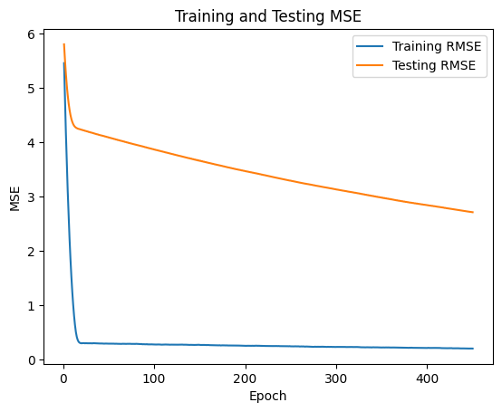
The following graph shows the training curve for the network. In the interest of time, I cut the training off at 450 epochs. The performance of the holdout test set was still improving at that point.
Discussion
The MovieLens dataset contains 943 users and 1682 items. Clearly, this is a pretty small dataset. There have been a number of different approaches to dealing with this problem including the release of the Torchrec domain library for Pytorch. Torchrec provides a way to handle embeddings such that they can be better parallelized across multiple machines. This allows network training to be scaled up to account for larger and larger datasets. In 2019, Meta (the parent company of Facebook) released an open source solution for dealing with the problem. Information about that approach can be found here.
Conclusion
In this post, I have discussed implementing a neural network based recommender system. I discussed, at a high level, how the neural network approach in this post differs from the singular value decomposition approach that I covered in my previous post. I included some examples of the network architecture both in it’s basic form, and with an added “bias” feature vector. I included code written in Python that uses the pytorch framework and that can leverage a GPU. I shared some initial results of the code showing how the network performed on a random hold-out test set. Finally, I included a short discussion on directions for neural network based recommender systems.
I hope you have enjoyed this post! Until next time…
Miles