Something Random

Recently, I came across a (very short) book by Andy Weir called Randomize. You can get if for free from Amazon. I won’t spoil it for you, but a main theme in the book is random numbers… or really the illusion of random numbers when it comes to computers.
When I was reading this book (short story might be a better description), it occurred to me that infinity is to calculus what randomness is to statistics and probability. To clarify, being able to compute integrals and derivatives require the ability to handle and manipulate calculations involving infinity. In probability and statistics, we are often faced with random variables, and chance. In order to compute probabilities and confidences, we must be able to handle and manipulate calculations involving randomness, and random distributions of various types. And, just as in calculus and mathematical analysis where we have different kinds of infinity (countable vs uncountable), there are also different kinds of distributions of random numbers.
Not All Random is the Same
Statistics is the study of the properties of samples and using that information to make statements about populations. When people say “Pick a random number between 1 and 100…”, what they typically mean is to pick an integer between 1 and 100, inclusive, where each number has the same chance of being chosen. It turns out that there are other ways to pick random numbers, however. Consider this variation on the “Pick a number between 1 and 100 game.”
Pick 30 random numbers between 1 and 100, and compute their average and do that over and over again 100 times and write down the averages.” The list that you write down will be random… but it is a special kind of random. The Central Limit Theorem of statistics tells us that the list of 100 averages will follow a normal distribution. (The CLT requires that the samples must have a sufficiently large sample size, usually n>=30.)
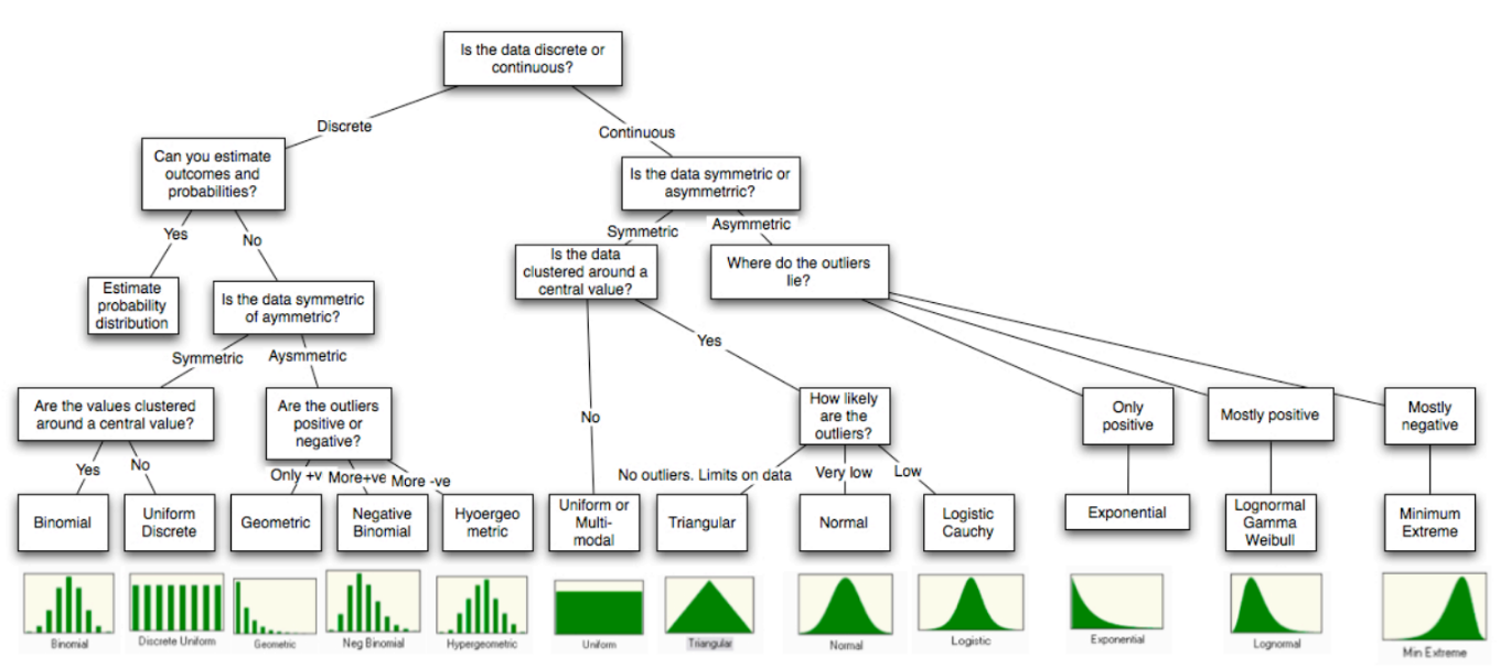
What we are touching on here is the idea of distributions of random numbers. If I say pick a random number between 1 and 100, that is called a “uniform” distribution. However, when I look at the means, I am starting to approximate a different kind of random distribution called a “normal distribution”. There are many other kinds of random distributions.
Stochastic vs Deterministic
Random numbers underlie the concept of stochastic models and optimization. Random, or “stochastic” models stand in contrast to what is often referred to as “deterministic” models, which use a direct approach. To understand the difference, consider two methods for estimating Pi. The method that Archimedes used, which involves circumscribing triangles inside of a circle would be considered deterministic. In the Archimedes algorithm, you don’t need any kind of randomness to do the calculations.
In contrast, the so-called “Monte Carlo” method involves randomly adding dots to a square with a circle enclosed inside.
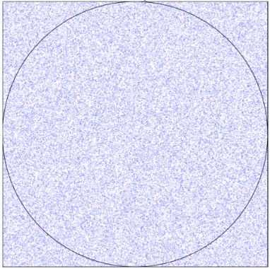
In this approach, you add as many random dots as you would like, and then count those that fall inside the circle. You can then use this formula to get an estimate for Pi.
\[\pi \approx 4 ( \frac {num\_points\_in\_circle} {total\_num\_points})\]This approach is considered stochastic as it requires the use of random numbers for the simulation to work.
Good Random vs Bad Random
“True” random numbers are not predictable. Also, sequences of true random numbers are not generally repeatable on demand. Stochastic algorithms would not be repeatable if they relied on truly random numbers. And, without repeatability, algorithms that use stochastic processes would be very difficult to test and results would be impossible to confirm.
Digital computers are deterministic machines. Digital circuitry alone is not capable of creating truly random numbers (unless it is malfunctioning). Nature, however, is full of sources of randomness. To come up with true random numbers computers use devices called true random number generators or TRNGs. These devices usually involve some physical and analog source of entropy. True random number generators play a critical role when it comes to cybersecurity. An interesting example of one elaborate TRNG was created by the cybersecurity company Cloudflare in 2017. You can read more about it here. For simplicity, speed and repeatability, computers typically rely on algorithms called pseudo-random number generators, often called PRNGs. PRNGs involve a random seed to start with. We will see some examples next.
IBM developed a PRNG in the late 1960s called RANDU. This once highly regarded PRNG used this formula:
\[V_{j+1} = V_j mod 2^{31}\]Known as a linear congruential generator, or LCG, the above sequence provides seemingly random numbers as shown below (scaled to between 0 and 1).
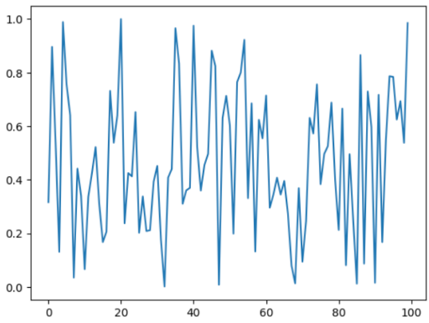
One advantage of RANDU was that it was very fast to compute. However, to see the weakness of RANDU, consider each three consecutive values as coordinates in 3 dimensional space. The following animation shows the obvious issue RANDU has.
In addition to the clearly anti-random 3-dimensional distribution of RANDU, the PRNG also suffers from other issues. The following article does into detail on examining RANDU.
https://bkamins.github.io/julialang/2020/12/31/randu.html
Randomness and Regression
Randomness and normal random variables play an important role in regression, particularly when it comes to goodness of fit. Simple linear regression can be thought of as a best fit line thru a collection of datapoints.
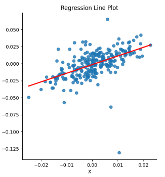
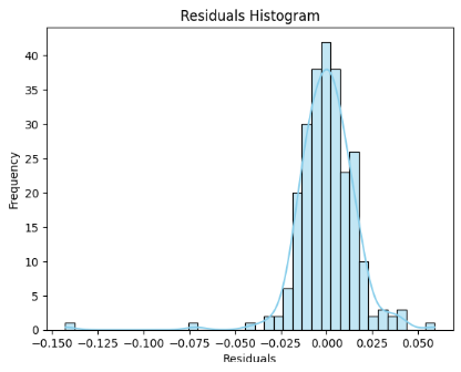
When we do a regression, one of the things that we pay special attention to is the difference between the original data points that we are trying to fit a line thru, and the difference between those points and the best fit line. These differences are referred to as the “residuals”. When we do regression, if we can show that the residuals are normally distributed, it opens up the opportunity to make statements about how well our regression line fits our data. To make our statements, we need the residuals to be independent from each other and all the residuals need to follow the same distribution. If this happens, we can state how well we expect our regression model to do in inference. This, by extension, makes it possible for us to create confidence intervals around our regression line. Having a “well fit model” also makes it possible for us to make statements about our confidence in the values of our regression model coefficients.
Random Means Not Predictable
At Georgia Tech, I took a class on business analytics. It was an interesting, if not a bit scattered course, that covered aspects of finance, digital marketing, and a number of other topics. One of the best things about the class was the book… that we never used. (Not sure why.) The book was “Data Mining for Business Analytics”. ISBN: 978-1-118-87936-8 by Shmueli, Bruce, Yahav, Patel, and Lichtendahl.
Towards the end of the book, there is this quote… “Before attempting to forecast a time series, it is important to determine whether it is predictable, in the sense that its past can be used to predict its future beyond the naive forecast.”
In other words, sometimes things are just random based on what you know. DON’T WASTE TIME TRYING TO PREDICT THEM!
A time series where each term is the previous term plus some random noise is known as a “random walk”.
\[X_{n} = X_{n-1} + \epsilon\]It turns out that there is a really easy technique to determine if a time series is a random walk, which involves fitting an AR(1) model. An AR(1) model (or ARIMA(1,0,0)) is simply a regression model where each term in the sequence is regressed back on the previous term. In other words, take all the pairs in the time series defined by:
\[(X_n, X_{n-1})\]If the slope of a regression line fit to the above pairs is 1, we have shown that the sequence is a random walk. Since this is a regression model under the hood, we can also look at the P-value for the coefficient in the underlying model to get a sense of how reliable that coefficient is. As we mentioned before, making those “goodness of fit” statements relies on the fact that the residuals are independent and identically distributed. While the values in our time series are NOT independent (each step in the time series depends on the last one), the difference between two successive steps should be. To see why, look at the definition of a random walk, and move the $ X_{n-1} $ term to the left side of the equation.
\[X_n - X_{n-1} = \epsilon\]In the above, $ \epsilon $ represents random noise.
An Example
Here is an interesting example. Below, I have taken the daily closing values of a company’s stock from Jan 1, 2021 thru Oct 10, 2023.
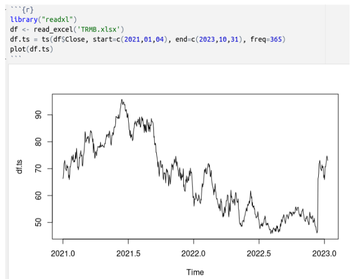
Next, using the R programming language, I have fit an ARIMA(1,0,0) model (aka AR(1) as mentioned above) to the data.
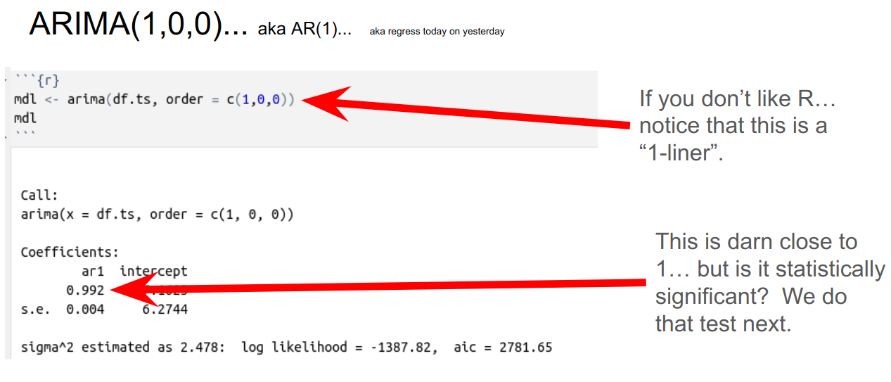
As illustrated above, the coefficient is really close to 1. Continuing on to check the statistical reliability of the coefficient in the model, the P-value is nearly zero. This means that the coefficient is highly reliable and we are looking at a random walk.
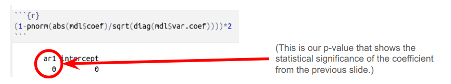
The bottom line here is that we have shown the stock above to be an essentially unpredictable random walk. Any efforts to fit a model based on JUST THIS DATA is not going to work. Now, that does not necessarily mean that we couldn’t find a different model with different predictor variables. It just means that the sequence itself is not enough to go on when trying to do predictions.
Conclusion
So, the takeaways from this post are:
- Random is to stats what infinity is to calculus.
- There are good random (estimate pi and lava lamps) and bad random RANDU.
- There are different kinds of random (distributions).
- Randomness underlies our ability to state the statistical significance and confidence intervals of regression.
- Some stuff is just random, so don’t waste your time trying to predict it.
I hope you have enjoyed this long overdue post. I wish everyone a wonderful holiday season, and a happy new year!