Reinforcement Learning meets Time Series Classification

What is past is prologue.  (Shakespeare, The Tempest, 1.2)

Introduction:

Everything that happens in our reality happens in the context of time. And, knowing some discrete or continuous measure of something is only meaningful in the context of when that measurement was taken. For example, consider $1000. That number means something very different today than it did in 1822. Because we exist, trapped in the constant flow of time, knowing what is comming next, or classifying what is happening in the present are highly valuable to us. It is of little wonder that finance, autonomy, and natural science are filled with problems related to time series analysis. It is ironic that, despite the fact that we live surrounded by problems involving time series, no uniform python packages have existed for time series modeling. While scikit-learn does offer some tools, those tools are very limited. In 2019, Franz Király, Markus Löning, Anthony Bagnall and Jason Lines began work on a python framework intended to follow the scikit-learn interfaces. Their framework includes tools and models for classification, forecasting, annotation, regression, and more. This post explores some of the tools provided in the sktime package for time series classification. It is worth noting that sktime goes far beyond just time series classification and includes tools for time series transformers, forecasting, and more.

Time Series Classification

So, what is time series classification? To begin with, we should probably define what a time series is. The term is almost completely self defining. In their book “Time Series Analysis and Its Applications” by Shumway and Stoffer (ISBN: 978-3-319-52452-8), the authors refer to time series as “…data that have been observed at different points in time.” (Note, the entire first chapter of this book is an excellent resource covering many topics and examples in this field of study.) A slightly more detailed definition comes from the NIST Engineering Statistics Handbook: “An ordered sequence of values of a variable at equally spaced time intervals.”

Mathematically, the definition of a time series can be written as:

$ y_t $ where $ t=(…-2,-1,0,1,2…) $

Source: Time Series Modelling, Inference and Forecasting by Prado and West.

According to Alexandra Amindon, Time series classification asks the question “Given a set of time series with class labels, can we train a model to accurately predict the class of new time series?” Amindon has written an excellent blog post on this subject on towardsdatascience.com.

Our goal here, however, is not to re-hash this excellent work, but rather to apply several time series classification algorithms offered by sktime on a particular time series classification problem.

Simulated Problem:

Time series classification, as the name implies, is a machine learning task that involves creating a model that can classify different time series into specific sets. In the movie, “The Hunt for Red October”, the characters in a submarine identify a sound made by another submarine. Their task is to identify the type of submarine based on the sound it makes. In this case, analyzing a discrete Fourier transformation of the sound would probably work well because the sound of the submarine propellers are very cyclic.

Now, let’s consider a different, and likely more difficult problem. What if we had a spaceship that was attempting to land on the surface of the moon. Our goal was to identify who was flying the spaceship based on the trajectory that the ship had while landing. This problem would be significantly more difficult than the submarine example simply because the trajectory would appear much more varied. To explore this specific problem further, it is possible to simulate the scenario of landing a spaceship on the moon, and training different “agents” as pilots.

Reinforcement Learning:

The OpenAI Gym provides a rich set of simulated environments that can be used to simulate/generate time series data. Once such environment is the “Lunar Lander” game. In this game, the goal is to safely land a simulated lander module on the surface of the moon. The simulation takes place in a simplified 2-Dimensional space. The game starts with a lunar lander module some distance above the surface of the moon. The player (agent) then uses thrusters (left, right, and up) to guide the lander to a pre-determined landing zone.

'AI Gym Lunar Lander'

For all those millennials out there, trust what many of us born before 1975 already know. The task is much harder than it sounds!

The objective of the OpenAI gym environment is to provide an environment that can be used to train reinforcement learning models. The reinforcement learning model used for this project is a Deep Queue Network or DQN.

It should be noted that, in this case, the DQNs fly the lander based on a parameterized subset of the environment “state”, which includes the location and angle of the lander. (Note that the lander will rotate when the lateral thrusters are applied). This approach of using parameterized values is somewhat different from other reinforcement learning models that use the graphical representation of the game “screen.” Using the parameterized values reduces the dimensionality of the problem space considerably, and reduces the time required to train the model.

The OpenAI Gym Lunar Lander code is part of the OpenAI Gym project and is opensource and freely available. More information about the PyTorch DQN is available on their website as well. While it would be tempting to dive into these resources further, we will continue to just focus on the time series data generated by the agents trained using these tools and techniques. Code for the neural networks is available at the link at the end of this post.

The Data

As missions are flown by the novice and expert agents, the state values of the game are saved. Each mission is saved as an individual file. Each of these files, then, can be thought of as a multidimensional time series. For the purposes of this paper, we looked specifically at just two parameters of the state, specifically the X and Y values of the lander. The goal of this paper was to focus just on univariant time series data. Therefore, it is necessary to take the X and Y values and somehow map them into a single value. In order to create this mapping, we first derive the velocity of the lander in the X and Y directions. Once the velocity has been calculated, the magnitude of the velocity M of the lander is calculated based on the simple formula

M = sqrt(X^2 + Y^2)

Where X and Y are the velocity in the X and Y directions.

It is possible to use the same approach on the change of the velocity of the lander. This, of course, is the lander’s acceleration. It is also possible to use the same approach on the change of acceleration of the lander. The change of acceleration is also commonly referred to as the “Jerk”. For this exercise, velocity returned the best results.

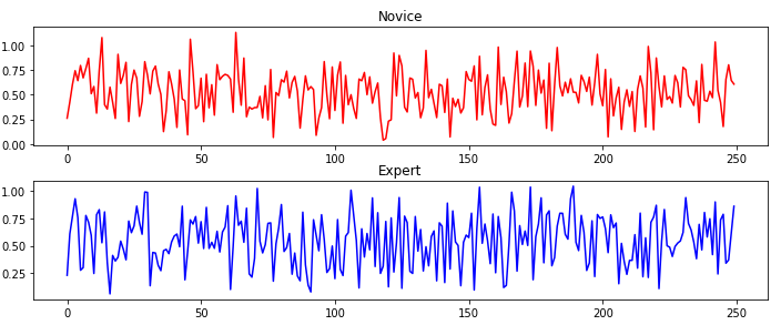
Here is an example of the velocity for a random novice and random expert flights. Here the novice flight was flown by an agent that had 300 epochs of training data vs the expert that that 700.

'Expert vs Novice'

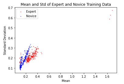
Another interesting visualization of the data is to look at the mean and standard deviation of the time series plotted on a graph where the x axis is the mean and the y axis is the standard deviation. Here, each dot represents one time series or “mission”.

'Expert vs Novice'

Once the data has been prepared for all of the agents, an 80%/20% train/test split will be used to divide up the data. While it would be possible to perform some type of cross validation on the data, the simple 80%/20% split will do for now.

The process:

For the proposes of comparison, the following classification techniques were considered:

IndividualBOSS
KNeighborsTimeSeriesClassifier
TimeSeriesForestClassifier
MrSEQLClassifier
MatrixProfileClassifier

The following code is the main cell in the jupyter notebook that is responsible for training and testing the different models. This code is also available in the URL mentioned at the end of this post.

from sktime.classification.all import ColumnEnsembleClassifier, RandomIntervalSpectralEnsemble, RandomIntervalSpectralEnsemble, IndividualBOSS, KNeighborsTimeSeriesClassifier, ShapeletTransformClassifier, MrSEQLClassifier
import sktime.classification.all
from sktime.classification.feature_based import MatrixProfileClassifier
from datetime import datetime

classifiers = ['IndividualBOSS', 
            'KNeighborsTimeSeriesClassifier', 
            'TimeSeriesForestClassifier', 
            'MrSEQLClassifier',
            'MatrixProfileClassifier']

def factory(classname):
    try:
        cls = getattr(sktime.classification.all, classname)
    except:  #Unfortunate kluge for matrix profiles.
        cls = getattr(sktime.classification.feature_based, classname)
    return cls()

for c in classifiers:
    _ = factory(c)


print("Classifiers appear to be present.")

results = []
for classifier_name in classifiers:
    start = datetime.now()
    print("Working on: {}".format(classifier_name))
    start = datetime.now()
    classifier = factory(classifier_name)
    
    # Train the model
    classifier.fit(X_train, y_train)
    
    trained_t = datetime.now()-start
    
    start = datetime.now()
    
    # Predict results on test data
    y_pred = classifier.predict(X_test)
    
    inference_t = datetime.now()-start
    
    # Measure accuracy of predictions against "ground" truth.
    a = accuracy_score(y_test, y_pred)
    
    # Save resultes
    results.append([classifier_name, trained_t.seconds/len(X_train), inference_t.seconds/len(X_test), a])

df = pd.DataFrame(data=results)
df.columns = ['Classifier', 'Training_Time', 'Inference_Time', 'Accuracy']

print("Models trained.  Results in tabular form:\n")
print(df)    

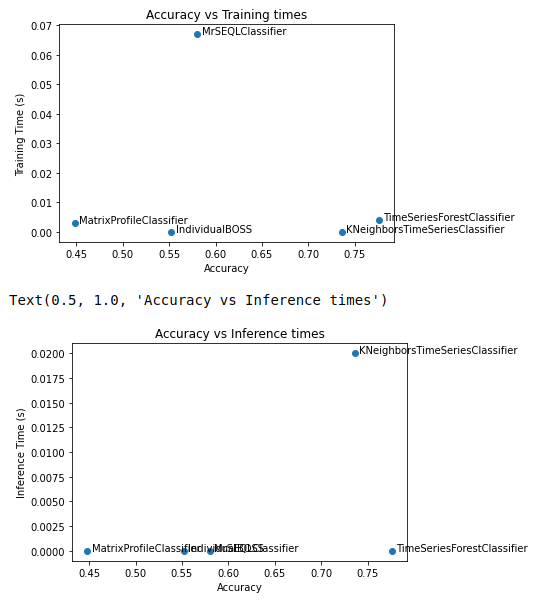
Results

The following is the results of the testing process:

                    Classifier  Training_Time  Inference_Time  Accuracy
                IndividualBOSS          0.000            0.00     0.544
KNeighborsTimeSeriesClassifier          0.000            0.02     0.736
    TimeSeriesForestClassifier          0.004            0.00     0.752
              MrSEQLClassifier          0.069            0.00     0.580
       MatrixProfileClassifier          0.003            0.00     0.448

If we limit the traning and testing to just the best and worst agents, the accuracies are actually much better:

                    Classifier  Training_Time  Inference_Time  Accuracy
                IndividualBOSS         0.0000             0.0      0.70
KNeighborsTimeSeriesClassifier         0.0000             0.0      0.84
    TimeSeriesForestClassifier         0.0000             0.0      0.86
              MrSEQLClassifier         0.0125             0.0      0.73
       MatrixProfileClassifier         0.0025             0.0      0.69

Conclusion

As can be seen from the above, the different time series classifiers in sktime offered different accuracies and different training and inference times. The TimeSeriesForestClassifier appeard to provide the best results for this dataset. Another interesting graph to consider in this experiment is the accuracy vs performance (training and inference time) for the different models.

'Accuracy vs Performance'

This experiment only scrapes the surface of the tools available in the sktime toolbox. I encourage you to check out sktime on your next time series project!

References:

https://www.frontiersin.org/articles/10.3389/frai.2021.699448/full
https://www.sktime.org/en/stable/

Source Code

Source code is available at the url below. (Note the jupyter notebook for timeseries analysis is in the /game/examples/agents directory.):

https://github.com/fractalbass/lunar_lander_ml