Principal Component Analysis

A Techical Review

Miles R. Porter

August 1, 2020

The purpose of this document is to review the concept of principal component analysis and how it relates to data analytics in general. This document will focus on the mathematical aspects of PCA, and will provide some references for implementing PCA for data analysis using python.

PCA is a technique for reducing the dimensionality of data sets. Dimensionality reduction is frequently used in data analytics to improve the performance of models (inference) as well as reduce the total amount of data needed to train a model. Consider the following motivational example of PCA.

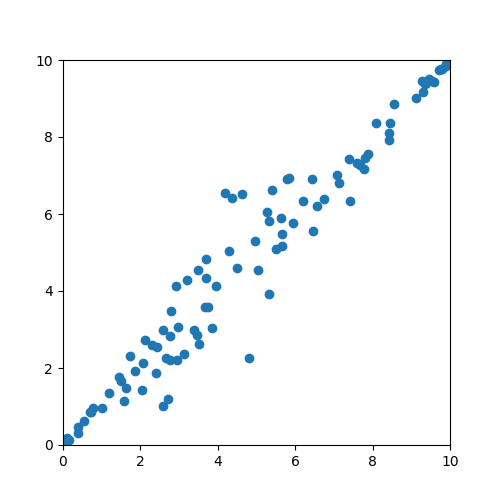
Intuitively, it seems like the data are lined up along a diagonal line. In other words, the primary dimensionality of this data is along the diagonal, and the secondary dimension of this data would be deviations from this diagonal. Consider the following image where these dimensions have been identified with red and green lines.

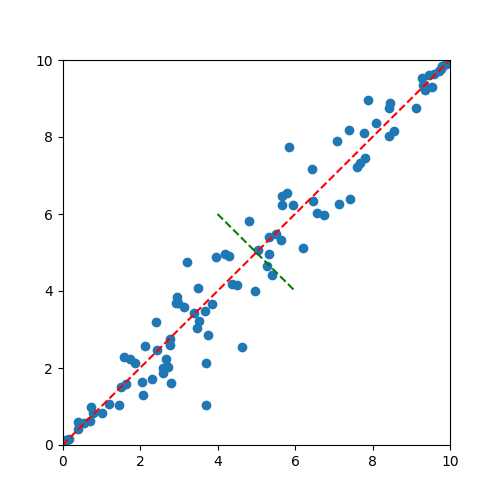
The above figure gives an intuitive feel for the goal of PCA, which is to identify the key dimensions that the data lay in. It is also important to note that in the above figure, the redline seems to capture most of the variance of the data, while the green line captures less. In this way, it is easy to see how we might consider the red line to be the primary principal component, and the green line a secondary component.

The above works well when considering data in only two dimensions, but what about higher dimensional data sets? To consider those aspects, it is important to think about the data from a more mathematical standpoint.

Moving Beyond 2 Dimensions

Consider the above example in two dimensions, but instead of thinking of the data as points on a plane think of them in matrix format, where each column of the matrix represents one of the points in the plane. Our data would then have 2 rows and 100 columns (short and very fat). The first few columns would look something like this:

\[\left[\begin{matrix} & 5.41 & 7.08 & 9.58 & 3.69 & ...\\ & 4.34 & 7.28 & 9.60 & 4.59 & ... \end{matrix}\right]\]

If we consider the above matrix to be X, then we can construct a linear transformation matrix P that transforms X into a new matrix Y. This can be described mathematically as follows:

\[PX=Y\]

Now, the columns of $X$, or the $x_i$ are our original data set. Likewise, the columns of $Y$, or the $y_i$ are our transformed data. Our goal in PCA is to come up with a matrix $P$ that transforms $X$ into $Y$. What we are after can be considered a “change of basis”.

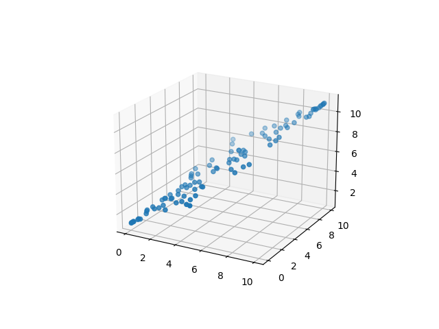
When we create the transformation matrix, we are going to want to accomplish a few things including finding and removing any unnecessary data. In the example above, it is clear that there are 2 dimensions that underly the data. If you imagine a third axis, it could be possible that we could reduce the data down to just two dimensions and still retain most of the valuable data. Figures 3a and 3b show a version of the above data in three dimensions. Here, clearly the Z axis is redundant as it represents very little new information that isn’t already present in the Y axis.

Figure 3a

![Figure 3b](/images/Figure_3b.png

Covariance

Covariance is a measure of the linear relationship between two variables. We can generalize this concept so that we have a covariance matrix which describes the covariance between all possible pairs of dimensions in a dataset. A covariance matrix can be computed as follows:

\[C_x=\frac{1}{n}XX^T\]

The above matrix $C_x$ is a symmetric MxM matrix and the diagonal of $C_x$ are the variance of the individual dimensions of the data. The off-diagonal terms of $C_x$ are the covariances between the different dimensions.

Now, if we can accomplish the following:

Find some orthonormal matrix $P$ in $Y=PX$ such that $C_y=\frac{1}{n}YY^t$ is a diagonal matrix, then the rows of $P$ are the principal components of $X$.

There are multiple ways to derive the matrix P above including eigenvector decomposition and a more general solution using singular value decomposition. For the purposes of this document, we will focus on the simpler eigenvector approach. Please refer to the endnotes for a reference to the SVD approach.

Eigenvector Decomposition

We would like to find some orthonormal matrix $P$ in $Y=PX$ such that $C_y=\frac{1}{n}YY^t$ is a diagonal matrix. In this case, the rows of P are the principal components of $X$.

\[C_y=\frac{1}{n}YY^T\] \[=\frac{1}{n}(PX)(PX)^T\] \[=\frac{1}{n}PXX^TP^T\] \[=P(\frac{1}{n}XX^T)P^T\] \[=PC_XP^T\]

It can be shown that any symmetric matrix $A$ is diagonalized by an orthogonal matrix of its eigenvectors. This can be denoted as:

\[A=EDE^T\]

Now, if we select a matrix P to be a matrix where each row $P_i$ is an eigenvector of $\frac{1}{n}XX^T$, we have $P\equiv E^T$. Furthermore, with that relation it can be shown that $P^{-1}=P^T$.

\[C_Y=PC_XP^T\] \[=P(EDE^T)P^T\] \[=P(P^TDP)P^T\] \[=(PP^T)D(PP^T)\] \[=(PP{-1})D(PP^{-1})\] \[C_Y=D\]

The above shows that with this choice of P, namely that it is a matrix where each column is an eigenvector of $\frac{1}{n}XX^T$, those eigenvectors are the principal components of our data X. Furthermore, for the matrix $C _y$, the entries on the diagonal are the variance of X along the $p_i$ component.

Calculating the PCA for a dataset, X, with python’s Numpy library is not too difficult. But, to make things even easier, the sklearn library for python makes the calculations very simple.

Sklearn Principal Component Analysis library

Utilizing that library, it is relatively easy to write python code to view the principal components of our data. Here is an example of the principal component analysis done using python on the data described above:

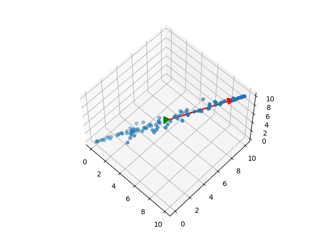
In the figure above, the red arrow indicates the principal component for this dataset. One thing to note about PCA is that once the principal components have been extracted, it is important to understand if they pertain to the new transformed space, or the original space. It is also important to keep in mind that if you transform data from a high dimensional space into a lower one, some information will be lost. It is possible to transform in reverse without loss of data only if all the principal components are used.

I have elected NOT to include code with this post for several reasons. The first of which is that I will be taking a course on computational data analytics and will likely want to reuse code I have developed for this blog post. There are, however, several good resources if you are interested in looking at specific implementations of PCA.