Comparing Neural Network Architectures for Voice Recognition
Introduction

I’ve been working on a recent Kaggle challenge that involves using TensorFlow for voice recognition. The challenge involves a large set of sound files that contains the words “on”, “off”, “stop”, “start”, “up”, “down”, “left”, “right”, “yes” and “no”. The files can also contain silence, or some other word not in the list above. In the case of other words, the challenge is to categorize these as “other”.
This challenge matches pretty closely the work that I did in this post on MFCC and HMM , except that TensorFlow and some type of neural network must be used to categorize the files rather than using hidden Markov models.
I am not completely done with the challenge yet, but have come across some interesting results in training the networks that I wanted to document in this blog post.
Voice Recognition with MFCC, a Brief Review
As I mentioned in my previous post on this topic, MFCC or Mel Frequency Capstrial Coefficients, are a common tool used when processing sound as part of speech recognition. This article, which I have referenced before, does an excellent job describing how MFCCs are computed. Without diving into too much detail, the MFCC technique can be used to convert audio into a spectrogram. Those spectrograms can then be used as input into a convolutional neural network and the networked trained to categorize the sound “images”.
Here is a sample image that was generated by using the MFCC tool python-speech-features created for python by James Lyons
Left:

Data Preprocessing
In order to make the images work a bit better, I decided to perform some basic cleanup. First of all, I decided that the images should all be of the shape(26,99,1). The first dimension 26, is the frequency “buckets” provided by the MFCC utility. The second dimension is the length of the file in terms of sample vectors. I decided that I would pad shorter files with 0s (see the code sample below). Secondly, I decided that the values for each pixel in the image should range from 0 to 255. The neural network code that I wrote uses Keras. Keras has a number of nice features for dealing with images including a “data_flow_from_directory” utility. This utility makes it easy to load and train networks based on a directory of image files. One thing that I would caution about is that it is easy to start to get confused about the dimensions of the image files used. Ultimately, the neural network definition and the evaluation data that you use all must agree in terms of the shape (dimensions) of the images. Keep in mind that the images must be represented in gray scale. If you don’t use gray scale images, that is fine, however that will mean that your images will need to contain additional dimensions that correspond to image channel colors. Also, the “99” dimension of the images corresponds to the time dimension. If the original audio files are shorter than 1 second, you will end up with images that are less than 99 pixels wide. To account for that, the code below starts with a zeroed out images of size 99x26, and copy the values from the converted audio file into that matrix.
Here is the main chuck of code that I used to pre-process the images…
from python_speech_features import logfbank
import scipy.io.wavfile as wav
import numpy as np

...

   def get_filter_bank_features(self, sound_file_path):
        (rate, sig) = wav.read(sound_file_path)
        filter_bank_features = logfbank(sig, rate, nfft=1600)
        if filter_bank_features.shape[0]<99 or filter_bank_features.shape[1]<26:
            print("Reshaping...")
            zeros = np.zeros((99,26), dtype=np.int32)
            zeros[:filter_bank_features.shape[0], :filter_bank_features.shape[1]] = filter_bank_features
            return zeros
        else:
            return filter_bank_features
Network Architectures
Links to the different architectures I have used on this challenge are below. I am not imbedding the images in this post to save space.
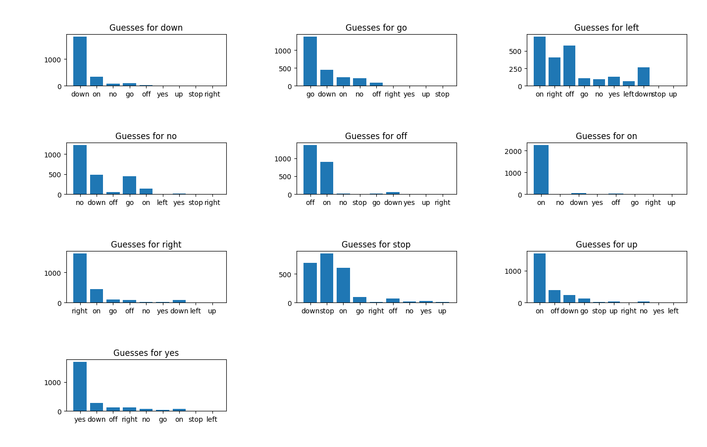
Results for the above networks can be seen below:
CIFAR-1
Network: CIFAR-1
Epochs: 100
Batch Size: 32
Training Time (sec): 1695
Training Accuracy: .8599
Training Curve: CIFAR-1
Final Accuracy: .5197

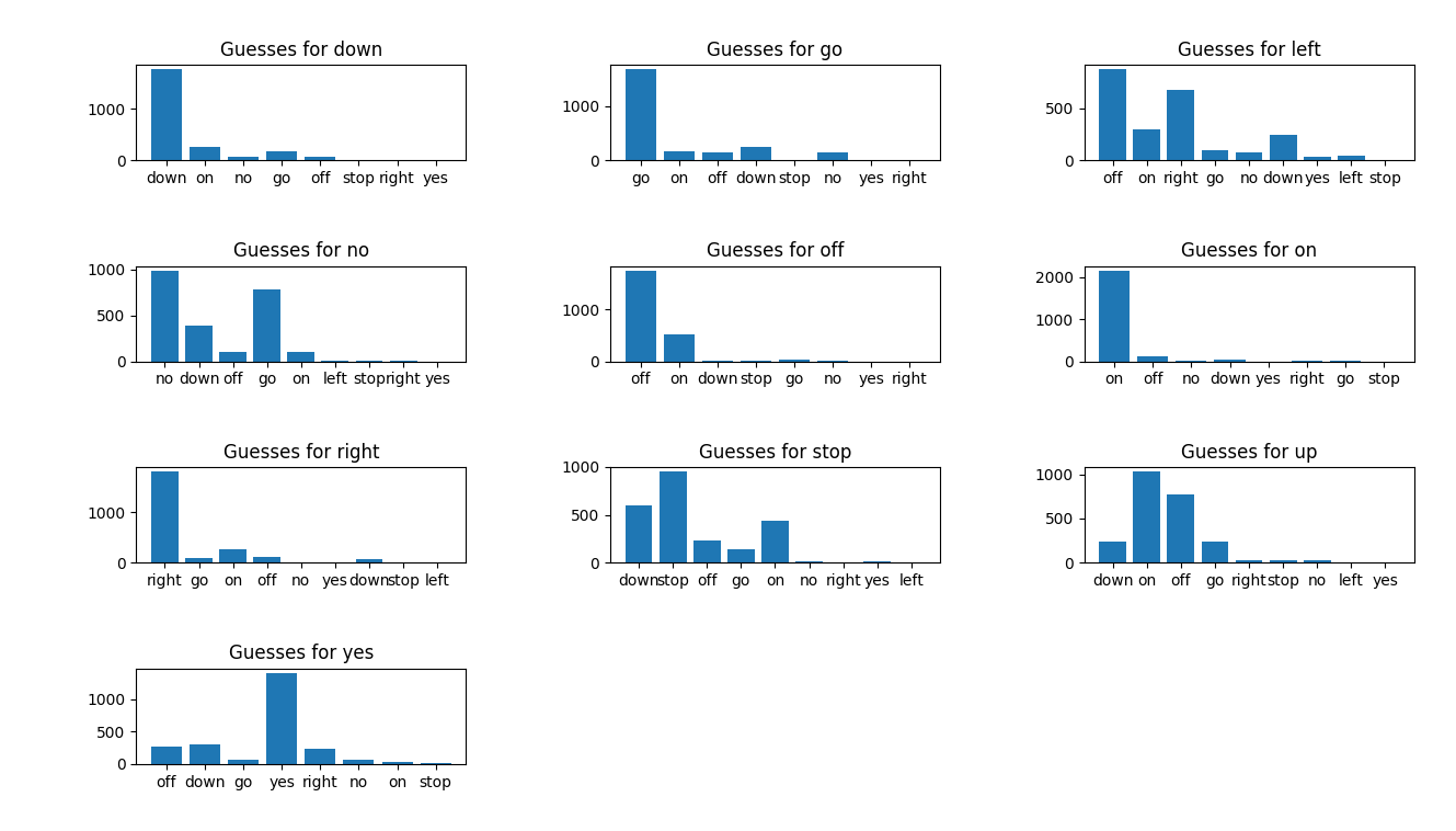
CIFAR-2
Network: CIFAR-2
Epochs: 100
Batch Size: 32
Training Time (sec): 2120
Training Accuracy: .8646
Training Curve: CIFAR-1
Final Accuracy: .5197

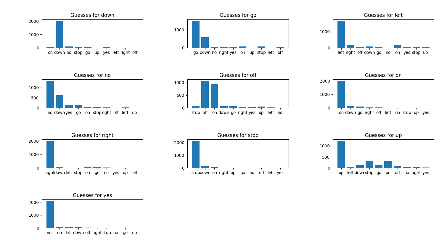
Analytics Vidhya 8 - 30 Test Paterns
Network: Analytics Vidhya Model
Epochs: 500
Training patterns: 10000
Batch Size: 32
Training Time (sec): 24195
Training Accuracy: . 8379
Training Curve: AV_Model
Final Accuracy: .7223

Conclusion
As you can see from the above trials, there are an infinite number of ways that we can architect the network to learn the data. Unfortunately, it seems like we can also spend an infinite amount of time trying to train the above networks! In order to make better use of my Mac, and go a bit easier on the machine itself, I have decided that this is a good time to wrap up this blog post and start looking into using the google cloud to train my models.
Stay tuned for that post…