Central Limit Theorem, Standard Deviation and Hadoop Combiners
Central Limit Theorem and Hadoop Combiners.

Paintchip Art by Peter Combe
Introduction
One of the fundamental concepts of statistics is the central limit theorem, which states:
If a sequence of Independent identically distributed random variables each has a finite variance, then as their number increases, their sum (or, equivalently their arithmetic mean) approaches a normally distributed random variable. (1)
In this post, we will explore the Central Limit Theorem, and a somewhat related phenomenon that relates to one of the quizzes of the Udacity Hadoop Mapreduce course. I believe that the course sets a pretty dangerous precedent with it’s very brief, and very wrong implementation of using a mean function as both a reducer and combiner.
The Central Limit Theorem
Let’s say that we have a population of 1000 values ranging from 0 to 100. Now, let’s say that I take a bunch of random samples of that population, with each sample consisting of 10 values.
The central limit theorem says that the distribution of the means of those samples will approximate a normal distribution. Also the distribution of the means will get closer to a normal distribution the more samples I take. Here is some code to illustrate this:
import random
import numpy as np
import matplotlib.pyplot as plt

nums = list()
num_of_samples = 10

#  Create a population of 1000 items
for i in range(0,1000):
    x = random.randint(0,100)
    print(x)
    nums.append(x)


#  Create samples.
sample_averages = list()
for i in range(0,num_of_samples):
    sample = random.sample(nums, 10)
    a = np.average(sample)
    print a
    sample_averages.append(a)
The above code creates my population of 1000 random values that range between 0 and 100. The code also draws 10 random samples, and computes the averages of those samples.
Now, let’s look at a histogram of the samples means (blue), and an approximation of what a normal distribution would look like based on the average and standard deviation of the sample means (red). First, the code:
mu = np.average(sample_averages)
sigma = np.std(sample_averages)

# the histogram of the data
n, bins, patches = plt.hist(sample_averages, 25, normed=True)
plt.plot(bins, 1/(sigma * np.sqrt(2 * np.pi)) *  np.exp( - (bins - mu)**2 / (2 * sigma**2) ), linewidth=2, color='r')
plt.xlabel('Average of Sample')
plt.ylabel('Count')
plt.title('Central Limit Theroem')
plt.show()
Here is the graph for 10 random samples…
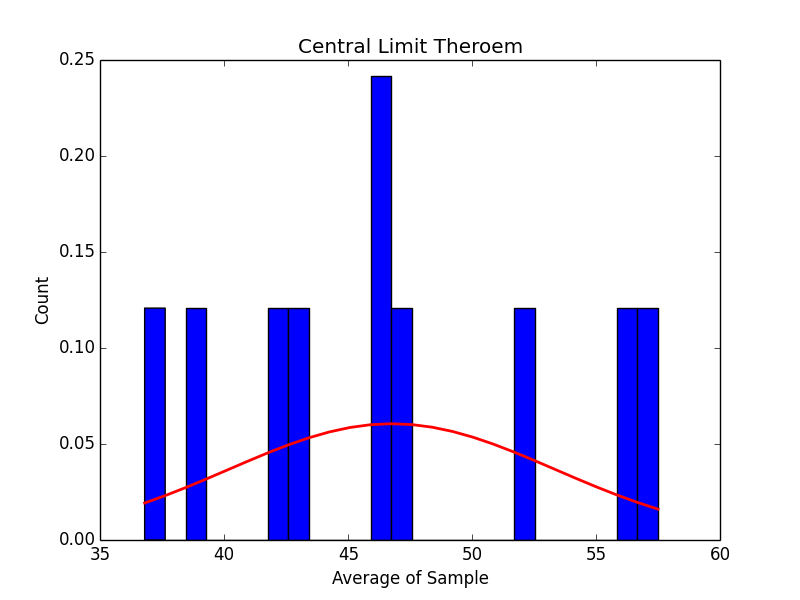
It doesn’t look like much, but as we increase the number of samples to 50, 250, 500 and 1000 we can start to see what the central limit theorem promises:
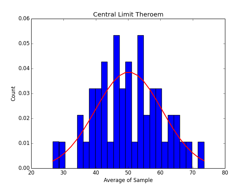
50 Samples:
250 Samples:
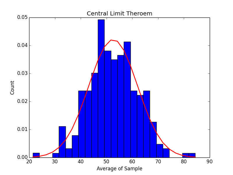
500 Samples:
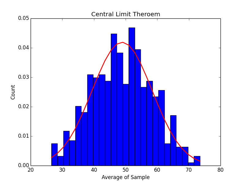
1000 Samples:
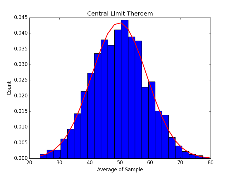
As the number of samples increases, our histogram does start to more and more closely match the graph of a normal distribution.
Keep in mind as we move forward that the number of samples that we take remains constant. We cannot have some samples of 10 items, some of 2, and some of 100. If we do that, the central limit theorem doesn’t apply, and all bets are off. Also, the central limit theorem only applies to the means of the samples. It doesn’t apply to the standard deviation.
Udacity Hadoop Combiners Quiz
I recently finished a quiz in the Udacity Hadoop MapReduce online course. The quiz was on combiners and basically focused on showing how using combiners can be used to optimize mapreduce jobs.
The quiz used a data set that contains product sales information. Each record in the set represents an individual item sold and includes, among other things, the cost of the item and the date. The exercise focuses on showing how computing the average sales by day of week can be optimized by using combiners.
This site contains a nice overview of what is going on with Hadoop combiners.
In the exercise, students are required to write a mapper that outputs each sale as the combination of a day of week as the key, and the value of the sale. My mapper looks like this:
class DOWMapper():

    logging.basicConfig(filename='mapper.log')
    days = ["Monday", "Tuesday", "Wednesday", "Thursday", "Friday", "Saturday", "Sunday"]
    sysin = sys.stdin
    sysout = sys.stdout

    def save_data(self, key, value):
        self.sysout.write("{0}\t{1}\n".format(key, value))

    def parse_date_amt(self, line):
        amt = None
        weekday = None
        try :
            fields = line.split('\t')
            weekday = datetime.strptime(fields[0], "%Y-%m-%d").weekday()
            amt = fields[4]
        except Exception as ex:
            logging.WARN("Error {0} raw data: {1}".format(ex.message, line))
        return self.days[weekday], float(amt)

    def map(self):

        for line in self.sysin:
            amt, weekday  = self.parse_date_amt(line)
            self.save_data(amt, weekday)

#Do the work
if __name__ == "__main__":
    mapper = DOWMapper()
    mapper.map()
Students are also required to write a reducer that computes the average value of the sales by each day of the week…
class DOWReducer():

    sysin = sys.stdin
    sysout = sys.stdout

    def save_data(self, key, value):
        self.sysout.write("{0}\t{1}\n".format(key, value))

    def get_average(self, l):
        total = 0
        for x in l:
            total = total + x
        return total/len(l)
...

    def reduce(self, q):
        result = None
        current_day = None
        day_sales = list()
        count_days = 0
        for line in self.sysin:
            fields = line.split()
            if len(fields) == 2:
                if current_day is None:
                    current_day = fields[0]

                if fields[0] != current_day:
                    #Done with this day.  Summarize and print
                    ave = self.get_average(day_sales)
                    self.save_data(current_day, ave)
                    if current_day == q:
                        result = ave
                    day_sales = [float(fields[1])]
                    current_day = fields[0]

                else:
                    day_sales.append(float(fields[1]))

        ave = self.get_average(day_sales)
        self.save_data(current_day, ave)
        if current_day == q:
            result = ave
        return result
You may wonder why I have written my own function to return an average. Keep in mind that I am dealing with python 2.6 because the Udacity virtual box image is running on an ancient version of CentOS. (See my previous post.)
At any rate, the mapper and reducer produce the following results:
Friday	250.223089314
Monday	250.009331149
Saturday	250.084703253
Sunday	249.946443251
Thursday	249.872024327
Tuesday	249.738227929
Wednesday	249.851167194
Again, this shows the average sales by the day of the week for the overall dataset.
The point of the exercise was to use the reducer as a combiner as well to improve performance. To see how that works, let’s first check out the number of input records that the reducer had to process for this job:

Mapreduce jobs consist of multiple mappers but only a single reducer. This can be an issue as it puts a lot of computation burden on the reducer. In order to get around that, combiners can be used. In the case of the quiz in Udacity, the student is asked to used the reducer as the combiner as well. The results of doing this are that the workload on the final reducer is much lighter and the job finishes more quickly.
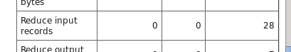
As you can see from the above screen shot, the reducer has a significantly smaller workload (28 vs 298,218) when running with combiners.
However, if we look at the resulting data we can see something pretty shocking… The result are actually different!
Friday	250.555395612
Monday	250.165178255
Saturday	250.248274952
Sunday	249.878222802
Thursday	249.707828286
Tuesday	249.614816971
Wednesday	249.640674892
What is happening?!
Essentially the combiner is acting as a sampler for the data, and the reducer is summarizing the data back from those samples.
Consider this example:
Let’s save I have a population of really boring numbers [1,2,3,4,5,6,7,8].
Now, let’s say that I break the data up into samples of different sizes. It just so happens that my samples cover the entire set and are not random, but that is fine. In fact it is exactly what the Hadoop combiner is doing; grouping up the results of the various mappers into samples.
Here are my samples:
[1,2], average = 1.5
[3], average = 3
[4,5,6], average = 5
[7,8], average = 7.5
Here the average of the sample means is 4.25. However, the average of the entire population is 4.5.
In the case of the Udacity quiz, we have no idea if the combiners are actually sampling the same number of records. If they were, we would be OK. But if the number of records in each subset is different, we cannot simply randomly split up our population into non-overlapping samples and then take “the mean of the mean” of those sample means and say that value is the same as the population mean. Well, I guess we could say that… but we would be wrong if we did.
The point of the exercise is to show that combiners can help reduce the bottleneck created by a single reducer. I get that. It still bothers me a little bit that what they were doing sets a bad precedent for a way to compute the population mean.
A Few Words About Standard Deviation
I had originally planned to look at the combiner quiz question, but use standard deviation rather than sample mean as the topic of this post. I did that because I thought that using a standard deviation reducer also as a combiner would cause problems. After thinking about it a bit, I realized that I didn’t even need to go that far.
If we take a moment and look at what happens if we try to compute standard deviation rather than sample mean we can see just how messed up this can get.
First off, let’s start with a test for calculating the standard deviation for values in a python list. Again, numpy would have made this trivial, but I am forced to run on Python 2.6, so no numpy. Grrr….
Anyway, here is a test:
    def test_reducer_stdev(self):
        reducer = Reducer()
        l = [1,2,3,4,5,6]
        stdev = reducer.get_stdev(l)
        self.assertTrue(stdev==1.707825127659933)
Is it a perfect test? No. But it will work for my purposes here.
Here is the code to satisfy the test:
    def get_stdev(self, l):
        total = 0.0
        for x in l:
            total = total + x
        a = total/len(l)
        v = 0.0
        for x in l:
            v = v + math.pow((a - x),2)

        stdev = math.sqrt(v/len(l))
        return stdev
One thing to note is that I have implemented the standard deviation of a population, not a sample. They are different. The population version of standard deviation is computed by first computing the variance for a set of data. The variance is the sum of the square of the difference of each value in the set to the mean. The standard deviation is then the square root of the variance. A sample standard deviation is computed by using a different formula. For more info on the difference between sample and population standard deviation check out this reference at statistics.leard.com
Now, when I use the above technique and compute the standard deviation of sales by day of week WITHOUT combiners, I get the following:
Friday	144.367101002
Monday	144.321171506
Saturday	144.401207177
Sunday	144.330561505
Thursday	144.339164506
Tuesday	144.205156383
Wednesday	144.255242005
Which is a dramatically different result than if we use the reducer also as a combiner:
Friday	62.4788765514
Monday	62.2390897986
Saturday	62.356315781
Sunday	62.3390116105
Thursday	62.3801593718
Tuesday	62.4122299749
Wednesday	62.2977859358
Conclusion
Hadoop combiners provide an excellent way to optimize results in map reduce jobs. That said, it is vital that data scientists and big data engineers keep in mind some of the basic rules of statistics when using combiners. The Udacity course only offers a very brief introduction to the topic, and they set a dangerous precedent for using combiners in conjunction with statistical methods for computing population means.
I hope you have enjoyed this exploration of statistics and Hadoop combiners. Stay tuned for more posts on data science, machine learning, and related topics.
My code for this post is available in github:
More Resources
- (1) Harper Collins Dictionary of Mathematics. ISBN 0-06-271525-9
- Statistics, The Exploration and Analysis of Data. ISBN 0-314-93172-4
- Leard.com Post on Standard Deviation
- calculator.net page for computing standard deviation
- Youtube video on Central Limit Theorem