Analyzing Audio Time Series Data with Fourier Analysis
Introduction
One of the key tools in analyzing data signals is the ability to break signals down into their component parts. Fourier Analysis is a technique that does just that. This blog post will cover some of the details of Fourier Analysis and the role that it can play in data science. A data scientist, albeit one without a sense of humor, would likely turn to Fourier Analysis to answer the question, “What is the difference between a saxophone and a lawnmower?”
Joseph Fourier
Jean-Baptiste Joseph Fourier was born in 1768 in Auxerre, France. Fourier was a man of many interests. He accompanied Napolean on his tour of Egypt and became a leading authority on the subject before and after Napolean’s rule.
Fourier’s contributions went far beyond his work in Egyptology. As part of his work in thermodynamics, Fourier developed an important technique that bears his name; the Fourier Series. Though untrusted by his peers at first, (they didn’t feel that he was rigorous enough in his work), Fourier’s technique for decomposition of periodic signals is a critical component of mathematical analysis, pattern analysis and signal processing.
A Brief Introduction to Fourier Series
A Fourier series can be defined as the following:
 (formula 1)
This form can be used to “… represent or approximate any single-valued periodic function by assigning suitable values to the coefficients.”
This series can be rewritten using complex values (complex as in imaginary numbers) as the following:
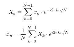 (formula 2 and 3)
Formula 2 just restates formula 1 using a bit of complex analysis. Formula 3 shows that the process is reversible. In other words, if you have the Fourier series, you can then get back to the original function. Enabling us to go back and forth between time domain and frequency domain views for the same function are what Fourier series are all about.
Kalid Azad has written an excellent post that explains how the Fourier series expansion (and the closely related Fourier transform) work. What better way to describe Fourier transforms, than in the context of smoothies?!
Fourier Transforms in Python
We will look at two ways to implement Fourier transforms using python. The first approach will start with an already existing sequence. In the second part, we will look at doing a little real-time analysis.
The Fourier series expresses a well known function into another function who’s coefficients correspond to the frequency breakdown of the original series. However, when we are dealing with recorded, digitized data, we don’t typically start with a well know function. In fact, much of the work with machine learning and predictive modeling is focused on getting to that point. We can still use the basic concepts that Fourier put forth. This technique is called the discrete Fourier transform or DFT.
If you are interested in the details of the DFT you can check out Wolfram Mathworld for more information.
One really nice thing about the python numpy library is that it provides a collection of methods for calculating the DFT from a given set of input points. The algorithm that numpy uses is referred to as the Fast Fourier transform, or FFT. (Hence the numpy.fft reference in the following code snippet.)
import matplotlib.pyplot as plt
import numpy as np

Fs = 150.0;  # sampling rate
Ts = 1.0/Fs; # sampling interval
t = np.arange(0,1,Ts) # time vector

ff = 5;   # frequency of the signal
y = np.sin(2*np.pi*ff*t)

n = len(y) # length of the signal
k = np.arange(n)
T = n/Fs
frq = k/T # two sides frequency range
frq = frq[range(int(n/2))] # one side frequency range

Y = np.fft.fft(y)/n # fft computing and normalization
Y = Y[range(int(n/2))]

fig, ax = plt.subplots(2, 1)
ax[0].plot(t,y)
ax[0].set_xlabel('Time')
ax[0].set_ylabel('Amplitude')
ax[1].plot(frq,abs(Y),'r') # plotting the spectrum
ax[1].set_xlabel('Freq (Hz)')
ax[1].set_ylabel('|Y(freq)|')

plt.show()
This simple little program draws up a graph of a sine wave, and then computes the discrete Fourier transform for that sine wave. When looking at the graph, we see a sine wave that does a little over 5 cycles in one second. The bottom graph is the DFT.
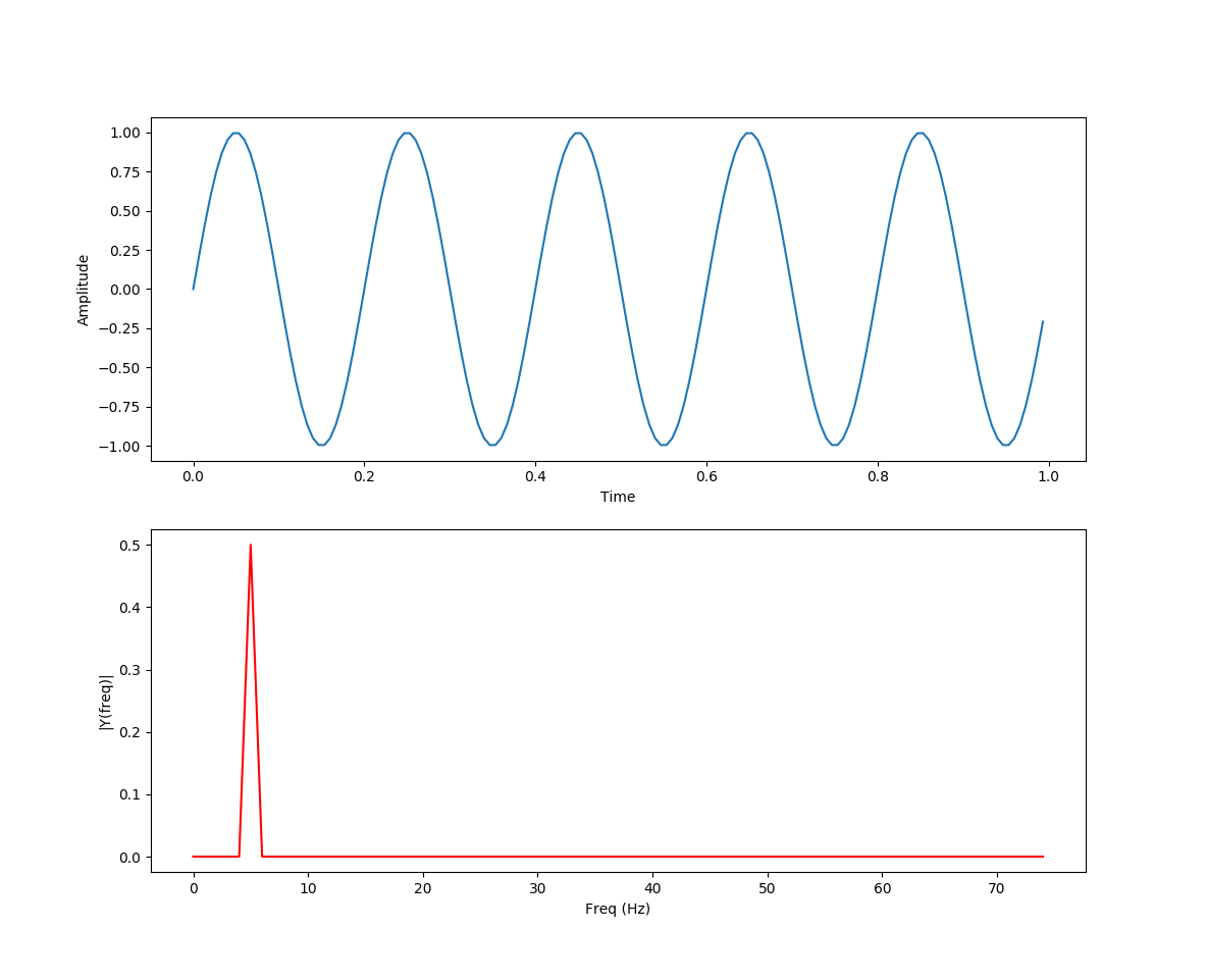
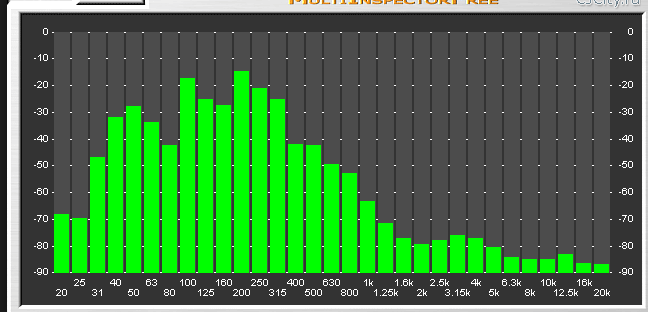
I like to think of that as a spectral decomposition of the top graph. The spike at somewhere around 5 (or a little less) corresponds to the number of waves in the above graph. Another way to think of this is the graphic equalizer display on old audio systems.
Going back to the python program, let’s make the function a bit more interesting by changing the following line…
...
y = np.sin(2*np.pi*ff*t)+0.3*np.cos(8*np.pi*ff*t)
...
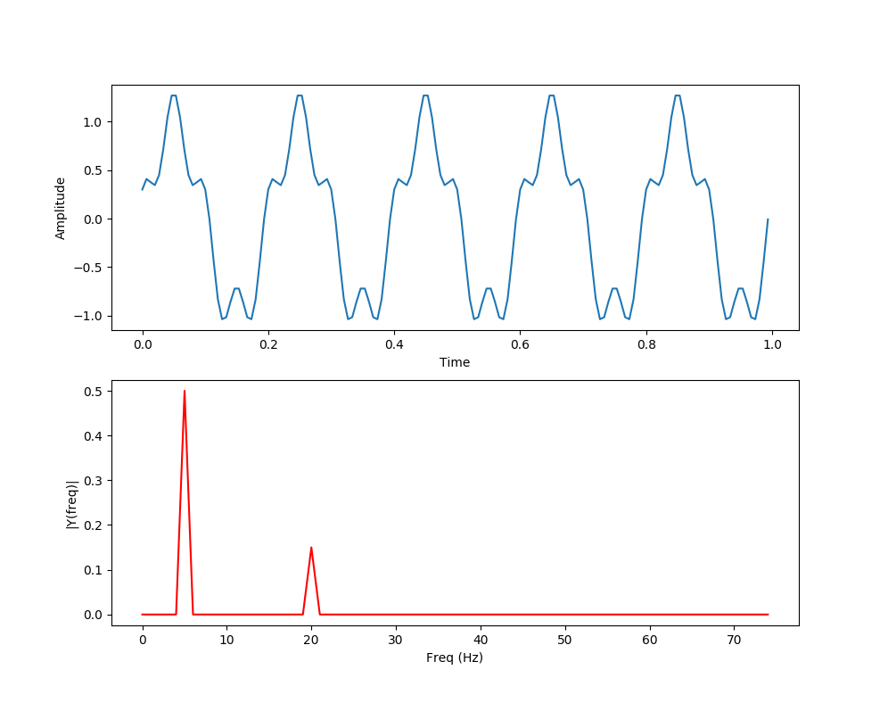
Here we can clearly see the main sine wave form that cycles around 5 times, and now we can also see the smaller cosine wave influence that cycles 20 times in the same 1 second.
Again, this is a highly contrived example. However, what would happen if we threw something really crazy at it like this:
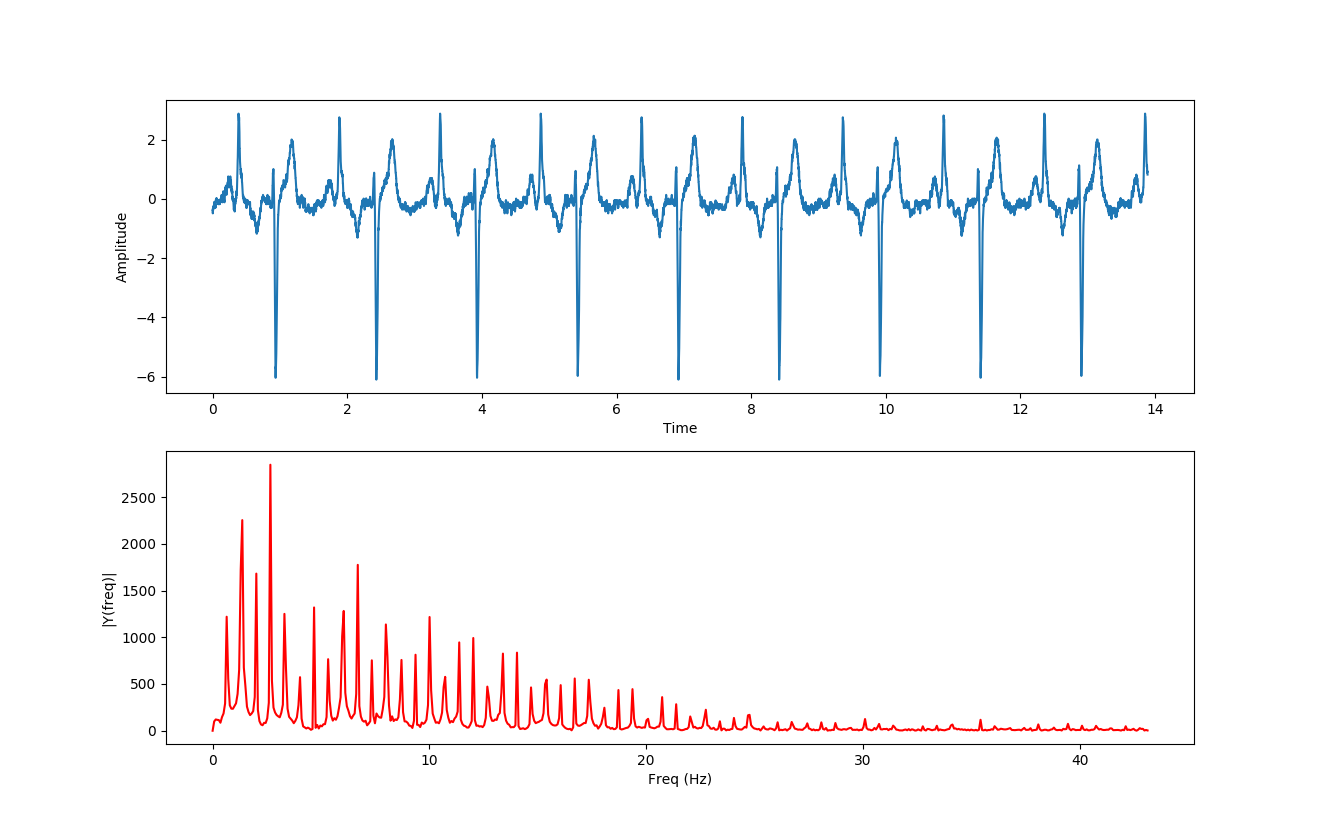
In this example, I have take an ECG waveform from The Physiobank website and ran it through the Fourier transformer that we had running before. You can see how the signature of the waveform is reflected in the frequencies identified by the FFT.
Note: EKG and ECG are interchangeable terms. I flipflop between the two without any reason, and I apologize to the reader if there is confusion. I will attempt to make sure that I stick with ECG, as it is closer to the actual term “Electrocardiogram”.
To see something really interesting and powerful, watch what happens if I offset the original way form by 2000 samples or 2.7 seconds:
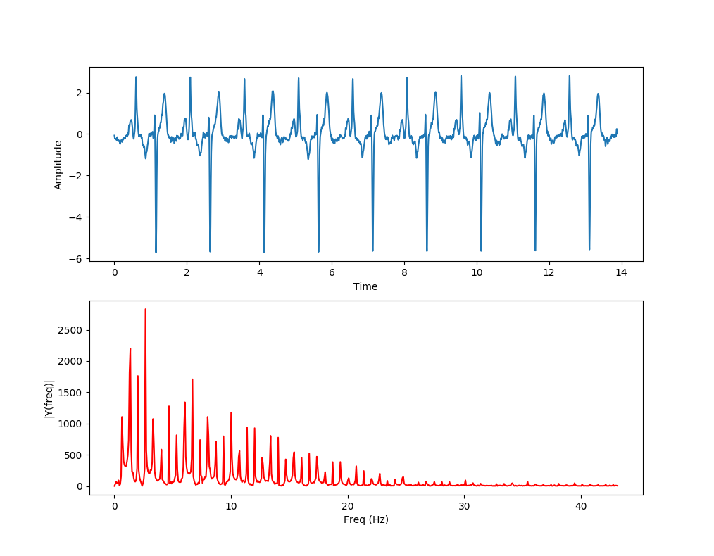
The data from the two transforms is identical (pretty much). Regardless of when the signal starts, the signature (the frequency decomposition, if you will) remains the same.
The advantage of using this type of analysis on repeating signals is that it is possible to use machine learning and other modeling techniques to classify data based on the FFT of the signal.
Analyzing the FFTs on stored data is useful. One nice thing about the FFT technique is that it is extremely fast. This means that it is possible to do this kind of frequency analysis in real time.
FFT in Real Time
The git repo for this blog post contains some code that performs realtime analysis of audio signals with a python program. The program was based on code from Florian Le Bourdais. I have modified his code in order to work with the newer PyQt5 libraries, which are a bit more mac-friendly than the earlier PyQt4 version.
The application that performs the realtime analysis is the LiveFFTWidget.py It looks something like this:
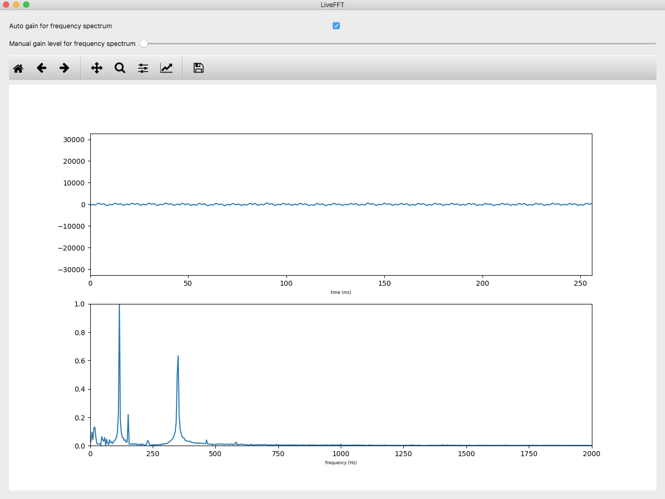
The wave on the top of the graph is the result of the microphone on my Mac picking up an “A” on my acoustic guitar. The frequency wave displayed below it shows that the note consists of two big frequencies at around 220Hz, and 440Hz. (That means that my A string is pretty well in tune BTW.) You will notice that there are 2 bumps, but I am only playing one note. The reason for this is that tones generated by the vibration of the string on the guitar doesn’t just consist of a single frequency. The series of other frequencies, and their relative strength is a big part of what makes different instruments sound differently.
To see a more complicated frequency breakdown, check this one out…
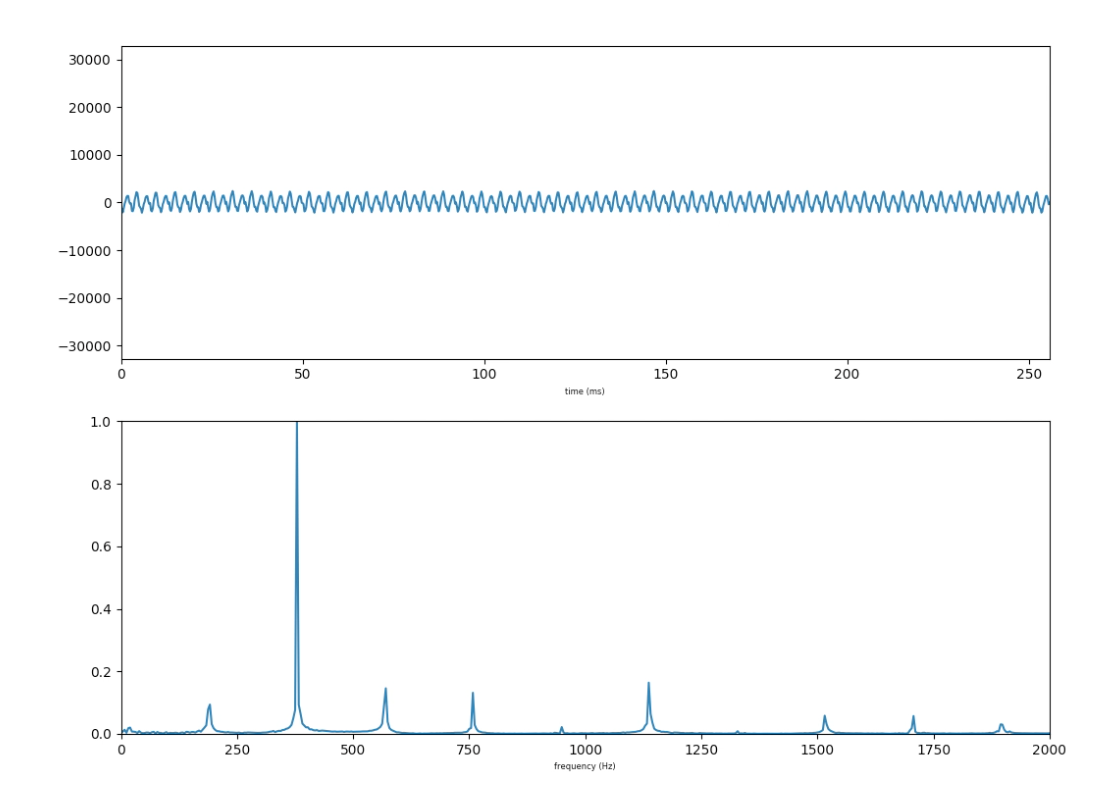 (figure 4)
This one has a frequency at around 440Hz, but several other bumps higher up in the sound spectrum.
Here is a really interesting one:
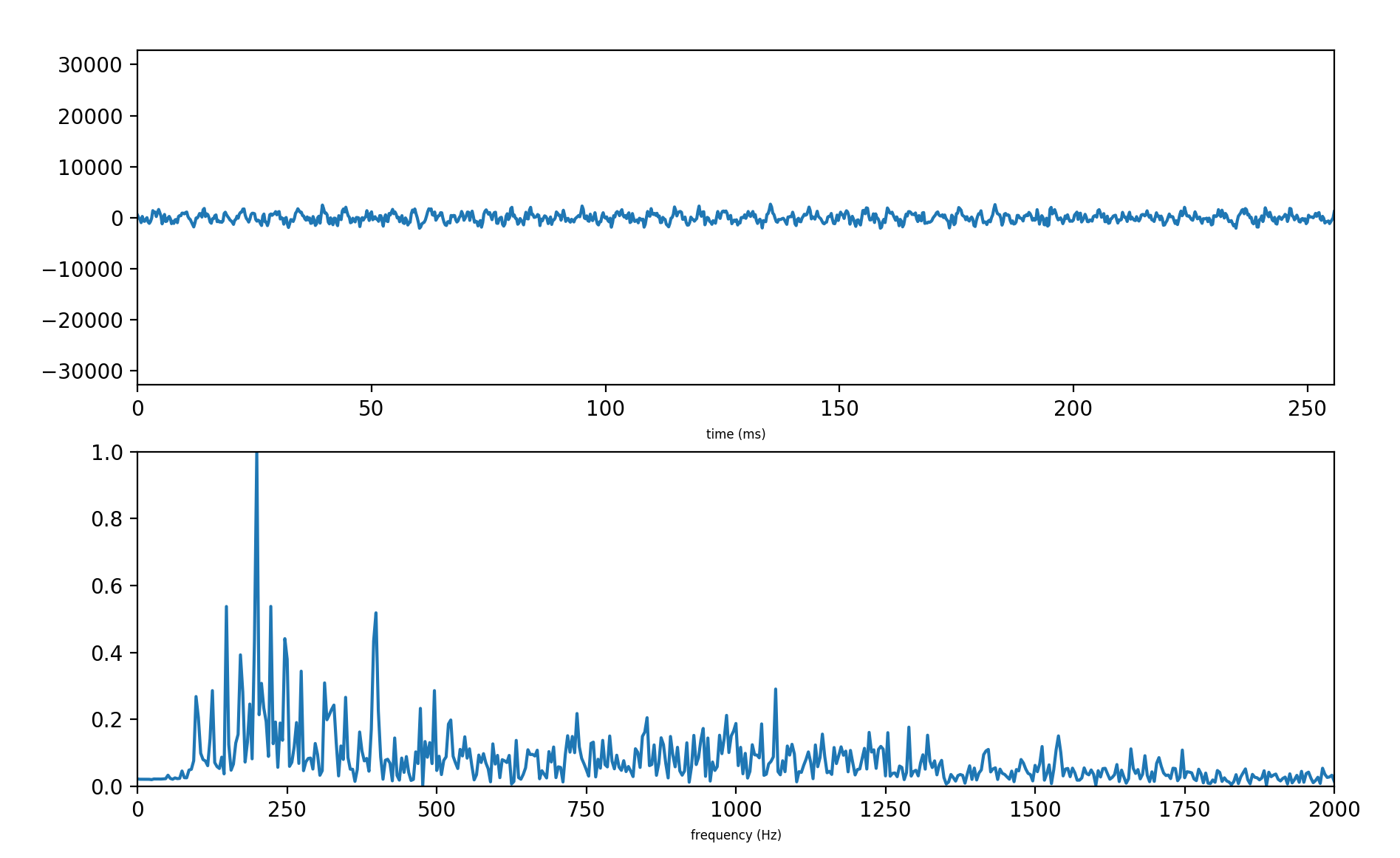 (figure 5)
This has a much more complicated signature, to be sure.
What were these two pairs of graphs (figure 4 and figure 5) generated by?
The first one is a saxophone and the second one is a lawnmower.
Despite what these graphs show, though, everyone knows that the real difference between a saxophone and a lawnmower is… wait for it…
You can tune a lawnmower.
(I’m hear all weak folks!)
Thanks for tuning in (so to speak) for this latest installment. Check back soon for more posts on topics in data science and machine learning. You never know what you’ll hear. (Ok. I need to stop now.)
References:
Encycploedia Britanica Online: Jean-Baptiste Joseph Fourier
Better Explained article on Fourier transforms
Boyer, Carl B. “A History of Mathematics” Princeton University Press, Princeton New Jersey, 1985. ISBN: 0-691-02391-3. Pg. 598-601
Borowski E.J & Borwein, J.M. “The Harper Collins Dictionary of Mathematics” Harper Collins, New York, 1991. ISBN: 0-06-271525-9. Pg. 228-229