Dedication

This is my happy place:

Bahia Honda State Park, Florida Keys.

I cannot help having a deep sense of dread that this lies literally just over the horizon:

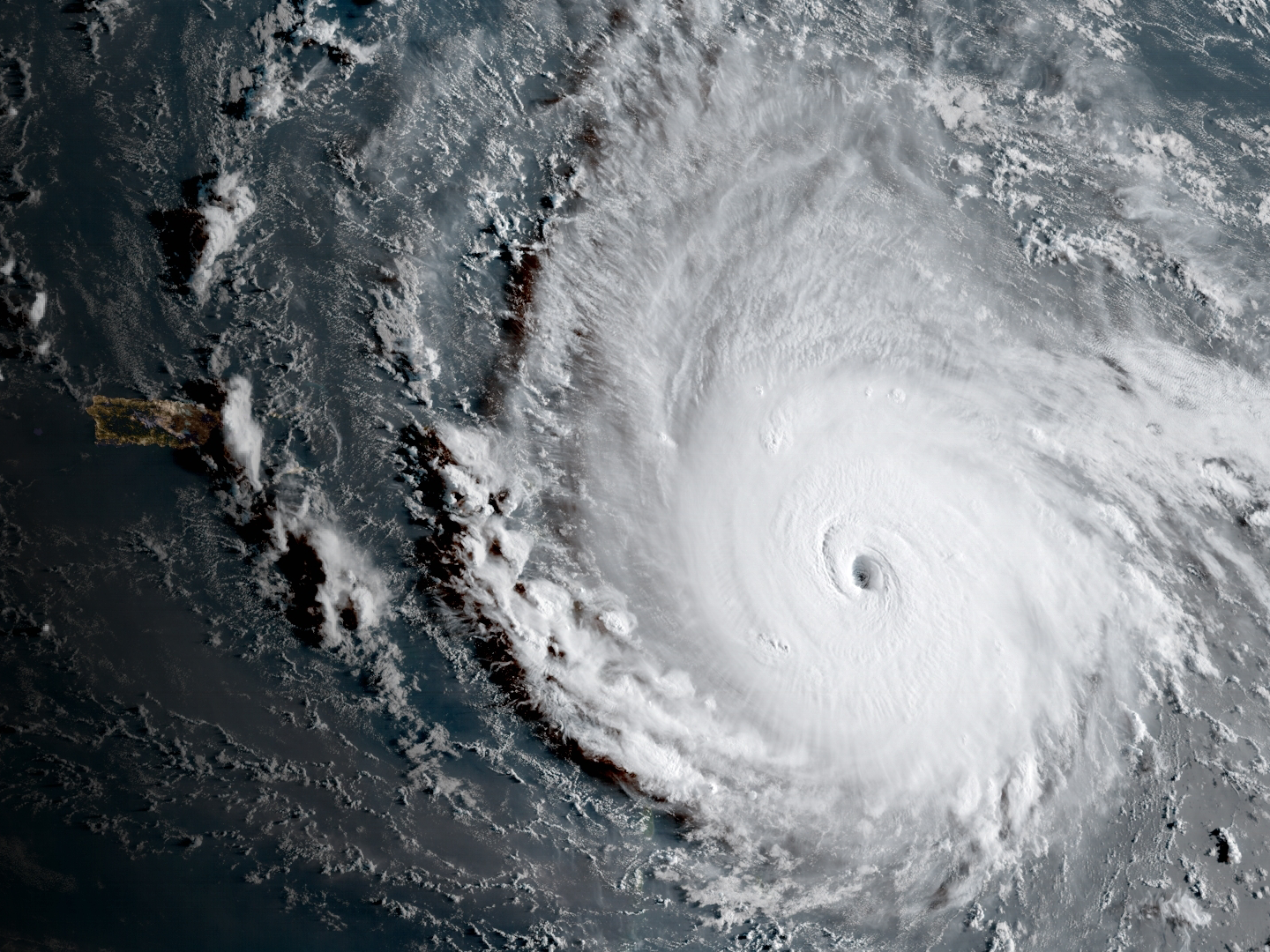
I sincerely hope and pray that the devastation that has smashed so much of the Caribbean will somehow miss the Florida Keys. I fear, however, that this “Strongest Hurricane On Record” may leave the island paradise forever changed.

It is one thing to sit and wait for the storm to impact a favorite vacation spot while the beauty of a Minnesota fall is starting to unfold right outside my window. But whatever dread and fear that I have is nothing compared to what the people, living in less than sturdy mobile housing in Marathon are feeling right now. I pray that they get out. I pray also that they have something to return to.

On Labor Day 1935, a category 5 hurricane struck the Keys. It was so strong, it blew train cars off their tracks.

Over 500 people died in that hurricane.

As bad as the 1935 storm was, Irma is even stronger.

This post is dedicated to everyone that has been or will be negatively impacted by Irma. My thoughts and prayers go out to all those affected by this storm, both in the keys and elsewhere. May you all stay safe and recover quickly from this cruel stroke of nature.

Why can’t we just predict the weather well in advance?

In the 1950s, John Von Neumann started designing computers at the Institute for Advanced Study at Princeton. One of the problems that he was hoping to solve was to come up with reliable long term weather prediction.(1)

Despite his best efforts and the work of others, long term weather prediction remained unsolvable.

Edward Lorenz, the original “Chaostician”

In the 1960s, Edward Lorenz, a mathematician and meteorologist at MIT was attempting to model the dynamic flow of the atmosphere with a computer that was different from Von Neumann’s; a Royal McBee.

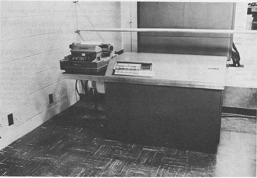
Lorenz used a computer like the one above to model fluid flow with a set of differential equations. Though Lorenz originally used 12 equations, the behavior that he discovered can be seen with a smaller set of just 3 equations.

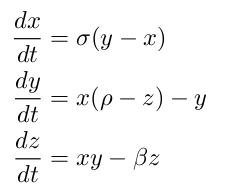
These three equations describe how a point in a fluid moves around when the fluid is heated from the bottom. The system of differential equations can be numerically solved by starting with an initial given point. From there, you can compute where that point will move based on the above equations. Once you have the new point, you can compute where the next point will be, and so on. There are a number of different implementations of this process in python readily available on the web. Here is one that I chose:

def lorenz(x, y, z, s=10, r=28, b=2.667):
    x_dot = s*(y - x)
    y_dot = r*x - y - x*z
    z_dot = x*y - b*z
    return x_dot, y_dot, z_dot


dt = 0.01
stepCnt = 10000

# Need one more for the initial values
xs = np.empty((stepCnt + 1,))
ys = np.empty((stepCnt + 1,))
zs = np.empty((stepCnt + 1,))

# Setting initial values
xs[0], ys[0], zs[0] = (0., 1., 1.05)

# Stepping through "time".
for i in range(stepCnt):
    # Derivatives of the X, Y, Z state
    x_dot, y_dot, z_dot = lorenz(xs[i], ys[i], zs[i])
    xs[i + 1] = xs[i] + (x_dot * dt)
    ys[i + 1] = ys[i] + (y_dot * dt)
    zs[i + 1] = zs[i] + (z_dot * dt)

fig = plt.figure()
ax = fig.gca(projection='3d')

ax.plot(xs, ys, zs, lw=0.5)
ax.set_xlabel("X Axis")
ax.set_ylabel("Y Axis")
ax.set_zlabel("Z Axis")
ax.set_title("Lorenz Attractor")

plt.show()

These lines of code result in the following plot.

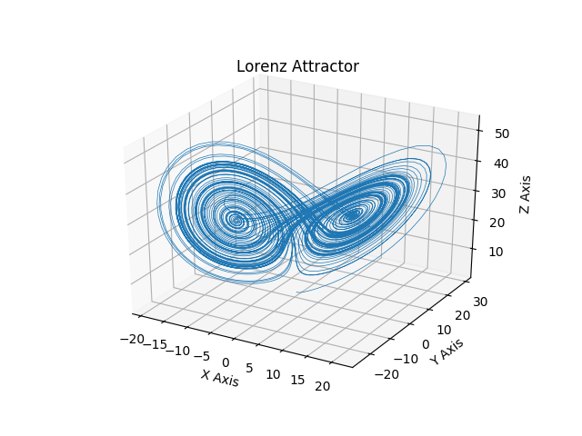
What Lorenz discovered is that if he started with a slightly different initial position, the system would end up in a completely different spot. To see this in action, I ran the Lorenz system of equations first with an initial point of:

(0.0, 1.0, 1.05)

Then I ran the equation again with a starting point of:

(0.0, 1.0, 1.0500000001)

Even with that very slight difference of 1 ten-billionth, the system ends up in a very different place.

1st Run: 9.709961879594102, 14.526677276746598, 21.237584691842496

2nd Run: -0.37938076506645446, -0.35531205260618304, 15.78002362694307

You can see how the sequences diverge when I plot the first one in blue and the second in red on the same graph:

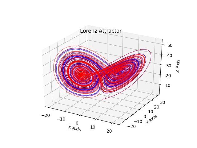
So, what does this mean for prediction? Because we can never have an exact set of initial conditions (our equipment is not infinitely accurate and we cannot measure every single point in the atmosphere) any type of prediction that we hope to have for the systems is eventually going to be wrong.

It’s not all bad, however. If I run the same experiment again, use points that differ by .001, and run out 800 time steps into the future, the graphs stay pretty close together. Using the second to predict the first is reasonably accurate.

1st Run: -9.354575653356267, -4.700936433736592, 33.034680891870465
2nd Run: -9.341238420532981, -3.464472307230002, 34.095203914473736

However, after just 100 time steps later the sequences have completely diverged.

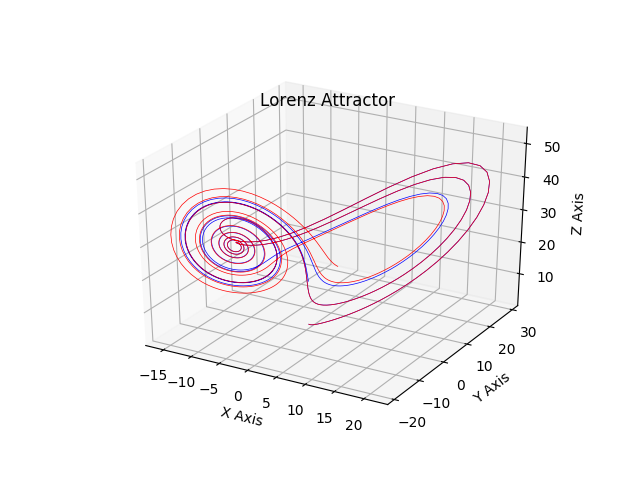
This shows us that we are able to model the systems fairly accurately in the short term, but over the long term, we just have no idea what the system is going to do.

Machine Learning and Dynamical Systems

It is tempting to think that we can get around this type of issue with some type of machine learning or data science approach. And, in fact, we are able to model these systems that way with some accuracy. Research has focused on using neural networks as a way to predict the behavior of chaotic systems.

But Ya’ Just Never Really Know

Unfortunately, one problem remains. Even if we were able to train a neural network or other type of modeling tool to accurately predict the behavior of chaotic systems like the Lorenz attractor, we could never get samples of data accurate enough to feed those models.

Conclusion

In this post we have looked that the behavior of chaotic systems, and specifically the Lorenz attractor. Machine learning tools like neural networks are able to model these systems with some level of initial accuracy, but eventually are unable to completely predict long term behaviors.

Code for this post can be found along with the code for the previous post in github.

References:

1. Gleich James, “Chaos, Making a New Science”. Viking Penguin, 1987. ISBN: 01400.92501 p.14

Wundeground Remembering the Labor Day Hurricane of 1935