“Every picture has its shadows
And it has some source of light
Blindness, blindness and sight”

– Joni Mitchell, Shadows and Light

Introduction

This is one of my favorite artifacts from the recent eclipse.

During the event, if you looked at the shadows made by trees, you could see lots of little eclipses projected on the ground. The effect is caused by the leaves of trees making pinhole lenses.

We can tell a lot about the situation looking at the shadows under the trees. There are also things that we cannot tell by looking at those shadows as well. With the powerful tools that we have at our disposal it is tempting to think that we can answer any question from any set of data. That is not, however, the case.

In most of my previous posts, I have looked at answering questions based on data. In this post, I am going to spend a little time musing about the situations when we cannot answer questions. Missing data, insufficient sampling, and utter randomness are all things that can block us from getting to some of the answers we seek.

Missing Dimensions in Data

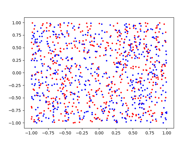
Consider the following plot of a dataset. The items in the set are color coded to belong to either the “red” or the “blue” class.

The goal of this exercise is to come up with a supervised learning algorithm that can learn to categorize points based on their coordinates. One approach to this kind of problem is to use a Random Forest model.

A Random Forest model, however, can return results that are somewhat misleading:

Calculation complete.  Random Forest Accuracy: 0.31

The accuracy indicates that the model is sometimes able to correctly predict a point’s category based on its coordinates. But, as the saying goes, “Even a broken clock is right twice a day.”

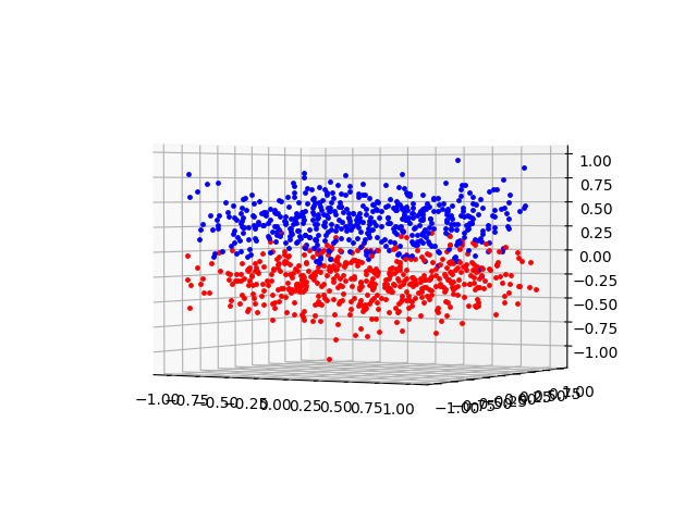
Let’s take a look at the data again… but this time, I will include a dimension that was not in the original set:

From this 3D plot, it is easier to see what is going on. The data for this dataset was created synthetically. Here are the key bits:

...        for i in range(0,500):
            x = -1 + (2 * random.random())
            y = -1 + (2 * random.random())
            z = random.normal(-3, 2) / 10
            ax2.scatter(x, y, c="r", s=6)
            ax3.scatter(x, y, z, c="r", s=6)
            data2d.append((x,y,"b"))

        for i in range(0, 500):
            x = -1 + (2 * random.random())
            y = -1 + (2 * random.random())
            z = random.normal(3, 2) / 10
            ax2.scatter(x, y, c="b", s=6)
            ax3.scatter(x, y, z, c="b", s=6)
            data2d.append((x,y,"r"))

As you can see from the above, the data consists of two groups of points in 3D space. The x and y coordinates of the points are randomly and uniformly distributed. The z coordinate of the points is also random, but the distribution is Gaussian (or Standard Normal, if you prefer). The red points are centered around z = -0.3 and the blue points are centered around z = +0.3. Running the analysis with this third dimension included in the data set results in an accuracy of 87%. If the size of the forest is increased from 100 to 1000, the accuracy increases to above 90%.

I think this is critical. The X and Y coordinates are basically just noise. There is no way that we could train any kind of model to learn to break the data apart. It would be sort of like trying to make a determination as to what the moon is made of by looking at the shadows under the eclipse tree. In both cases, we just don’t have enough information to make a determination. Yet, sometimes when we are faced with very noisy or difficult data, the temptation is pretty great to try to see patterns in what is essentially just static. The fact that the random forest is able to predict some of the data correctly (of course, it has a 50/50 chance) can easily lead us astray. Psychologically we want to come up with a model that works. All too often, I think, that can work against us.

A great exploration of this topic can be found in Neal Stephenson’s book Anathem. In the book, Diax’s Rake is “Never believe a thing simply because you want it to be true.” If you are curious about the details of Random Forest modeling, please see my previous post Seeing the Forest For the Trees for more details on that approach. The code associated with my posts are available on github.

Confidence Interval

The above example shows how a supervised machine learning algorithm can lead to some incorrect conclusions. In regular statistics, we can also make mistakes. Those types of errors can be broken down into three classes: First, we may fail to understand what we are doing with the data and apply incorrect formulas or distributions. Secondly, we can use the correct statistical formulas but interpret the data incorrectly. Finally, we may use the right tools, and understand the results, but we may simply not have enough data. Of course, if things are really bad, we can do all three; misread the results from the wrong formulas we got from bad or insufficient data.

I won’t go into using the wrong methods. However, lets look at an example where insufficient data and misreading results can cause problems. Consider this example: Let’s say that I have a yard that is somewhere around 15,000 square feet. I know for a fact that number is actually incorrect because I always buy the 15,000 square foot bag of fertilizer, and I ALWAYS have too much. Anyway…

In each square foot there is 144 * 47 blades of grass. (I know this from here.) So, based on this, my yard has roughly 101,520,000 blades of grass. If I measure 10 random blades of grass, I get the following:

Sample		Length(mm)
1		75
2		31
3		30
4		56
5		83
6		101
7		38
8		40
9		27
10		50
Mean		53.1
Var		643.21
Stdev		25.36

(Yes, I actually DID go pull 10 blades of grass from my yard.) In order to estimate the mean length of grass (the mean of the population) in my yard we could just say “It is around 53.1mm.” That would be ok and we could stop there… but that kind of effort is probably not going to get us a gig in data science. :)

To build a confidence interval estimate we would do the following. (Note: See this site for a nice explanation on the topic of confidence intervals on a sample mean.)

Sm = S / Sqrt(N) = 25.36 / 3.16 = 8.0253

Now that we have Sm, we need to look up the value of “t” for a T distribution where the degrees of freedom is 9, and for a 95% confidence interval. I used a table in the back of a very old stats book, but you could use this site. Either way, we should come up with:

t = 1.833

Finally, we compute our confidence interval to be:

Lower limit = 53.1 - (1.833)(8.0253) = 38.3896
Upper limit = 53.1 + (1.833)(8.0253) = 67.8104

And we could say that we are 95% confident that the mean of the population is between 38.3896mm and 67.8104mm.

But we won’t say that. Because if we did, WE WOULD BE COMPLETELY WRONG!

That is not what a confidence interval does. What we are really saying is that 95% of all samples of size 10 with a standard deviation of 25.36 and a mean of 53.1 will contain the population mean. Or, if we keep taking samples of 10, and we keep computing the interval based on the steps above, 95% of those intervals would contain the population mean.

An even easier way to think of this is… I took all the samples from my front yard (because I’m lazy and didn’t put on shoes and didn’t want to walk to the back.) The grass grows much taller in the back. Trust me on this. I mow my own yard and haven’t done it in a while. I know that the grass in the back is going to push the population mean much higher.

What have we shown here? Well, we don’t really have enough data to accurately make statements about the overall population. A single sample of 10 isn’t going to tell us much about a population of over a hundred million. Secondly, it can be very easy to misinterpret the results of confidence intervals.

Randomness vs Chaos vs Non-Linearity

I had intended for the last part of this blog to be about Randomness vs Chaos vs Non-linearity. However, I feel this post is getting to be a bit long. I will break that topic off into it’s own post.

Conclusion

In previous posts, I have focused on how to classify and make predictions based on data. This post touches on some areas where it is easy to mess things up. Looking for logic where there isn’t any, misunderstanding results and not using sufficient data when drawing conclusions are all things that data scientists need to be aware of when analyzing information.

I hope you have enjoyed this post. Please tune in next time for a deeper exploration into the topics of randomness, chaos and non-linearity.

Now, if you will excuse me, I am going to go put on some headphones and listen to Joni Mitchell while I mow my yard.

Credit where credit is due: Thanks, Paul Close, for noticing that I stupidly wrote centimeters when I really meant millimeters.