Introduction - The Paint Problem

I recently experienced a “watching paint dry” feeling… in a literal sense.

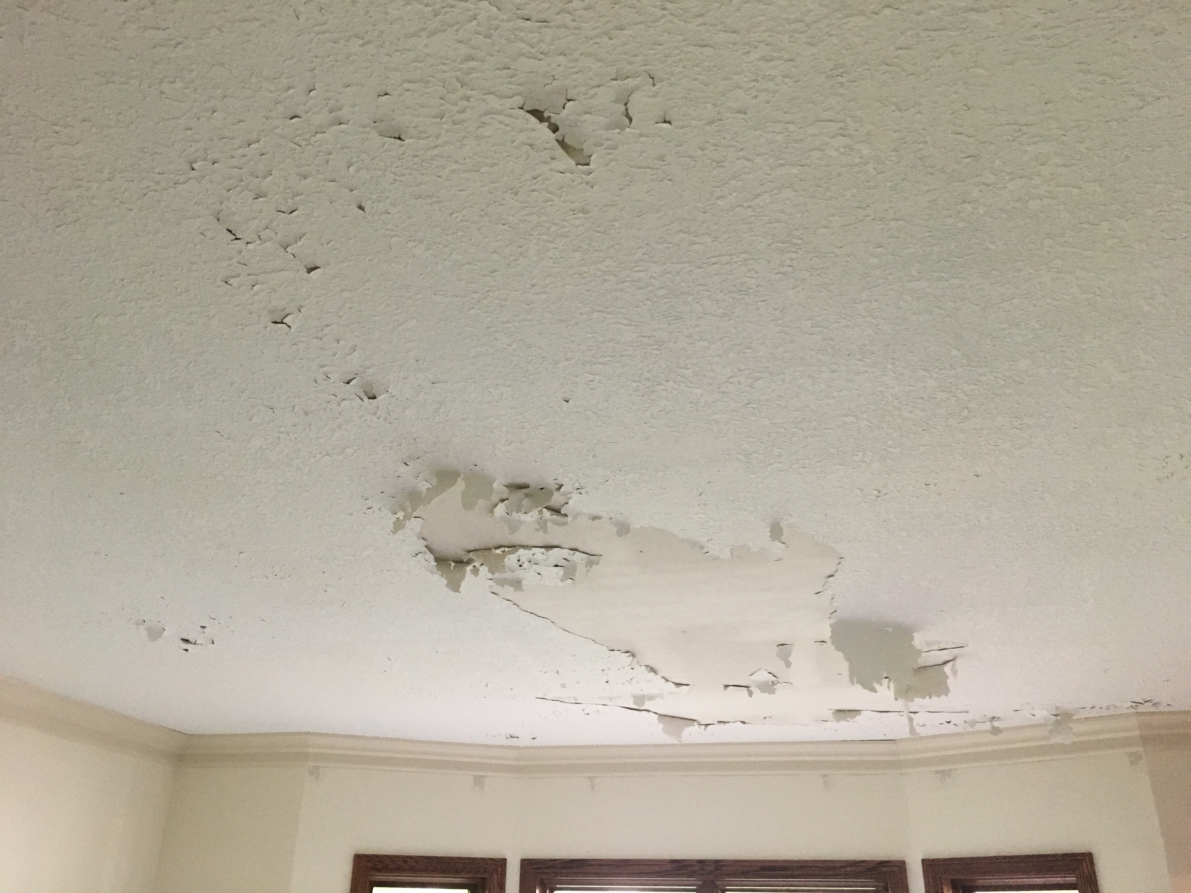
We just had some rooms in our house painted and our “popcorn” ceiling re-textured with “knock-down.” The end result is nice. The process involved with getting things to this state wasn’t.

The newly resurfaced ceiling started to peel just after the painters put a new coat of paint on it. After some head-scratching we realized that the humidity in the house seemed to be high. We were able to confirm this because of a little IoT project that has been up and running in the house for over a year. Check out the blog post about that project here.

The IoT project, which I presented on at the 2017 Embedded Software Conference in Minneapolis, employs Raspberry Pi based humidity and temperature sensors. The sensors forward their data to BeeBotte.com where the data can be viewed on a dashboard. The data from BeeBotte confirmed that when the painters attempted to paint the newly re-surfaced ceiling, the humidity in the house was unusually high.

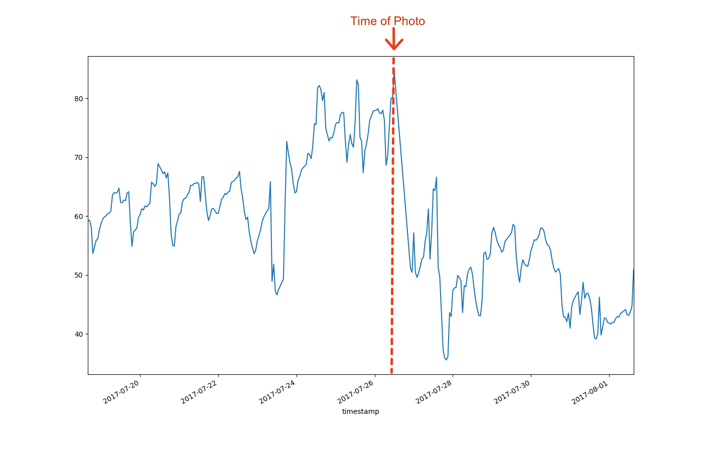
Humidity data in this graph is a time-series so it would seem that an LSTM could be a good tool to use to model the data. I touched on LSTMs in my last post. In this post, I will dig a bit deeper.

RNNs and LSTM Networks

A Recurrent Neural Network (RNN) is a neural network that attempts to “remember” data. There are a number of good resources on the web to read about RNNs including this blog post by Denny Britz. There are two key features to keep in mind about RNNs.

• RNNs act on sequences of training data. In other words, we don’t just past training patterns to RNNs to train them, we past sequences of training patterns.
• RNNs incorporate feed-back loops that pass data from the network back into it self.

Here is a diagram that shows how an RNN can be “unfolded” into a sequence of neural networks.

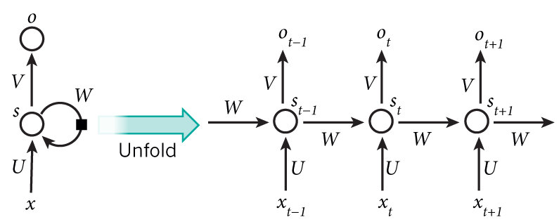
(The previous images was taken from Denny Britz’s Blog.)

• An LSTM is a special kind of recurrent neural network. A great explaination of LSTMs can be found in this blog post by Christopher Olah. It is important to note that any network that is trained by a gradient descent algorithm can potentially give rise to what is called the “vanishing gradient problem”. A good explanation of vanishing gradients can be found in this post by Nikhil Garg. Vanilla RNNs are particularly susceptible to this issue, and LSTMs are one technique to overcome vanishing gradients. You can read more about how LSTMs specifically attempt to address vanishing gradients in this post by Ottokar Tilk.

This, That and the Other Thing

When looking at this topic, I reviewed implementations from three main sources:

• Dr. Jason Brownlee’s post on time series forcasting
• Jakob Aungiers post on time series forcasting.
• Radix answer on this stack overflow post

In the end, I came up with a combined approach that is based a bit more on object oriented python, rather than python scripting. I used the Keras 2.0 running on top of TensorFlow.
The entire code for this post can be found in the GIT repository for this project.

Testing

While each of the resources mentioned above provided some value, I didn’t feel comfortable with the level of testing that seemed to be implemented with the code. This is a common issue that I have seen with a good deal of the work published on data-science and machine learning. I firmly believe that because machine learning techniques often deal with predicting data, it is imperative that good tests are used to ensure that the data involved is handled correctly. If there are errors in the way that we prepare the data, the value of the network is less than zero. I say that because, if the inputs to our network training contains errors, we end up training networks to predict the wrong thing. This situation can be summed up nicely with “garbage in - garbage out.” In order to protect against messing up the input data, I decided to write my own class with some basic level of testing to ensure that any pre-processing of data was being done correctly. I believe that this is especially critical for dealing with RNNs and LSTMs because a good bit of data manipulation must be done in order to set up and train the models. Check out my blog post on integration testing for a gentle introduction to unit and integration testing in python.

One of the benefits of writing unit and integration tests, is that it forces a developer to breakdown a problem into understandable units. You can see the results of this in top-level code for my implementation of the LSTM to model the humidity problem:

    def run(self):
        print("Starting...")
        # Load the note file
        file_helper = FileHelper()
        # new_file = file_helper.convert_dataset_file("./data/humidity_training_and_testing.json")
        new_file = "./data/sinewave.csv"
        print("New file {0} has been created.".format(new_file))

        rnn = RecurrentModel(seq_len=50, epochs=1000, use_differences=True, use_normalization=True, input_length=40,
                             output_length=10, training_record_ratio=0.5)

        rnn.prepare_data(new_file)

        # Train the model
        rnn.train_network()

        # Save the model
        rnn.save_model("{0}_model_{1}".format(new_file, datetime.now().timestamp()))

        # Display the graph
        rnn.display_results()

        print("Done.")

I think it is pretty clear from this portion of the main program as to what the program does:

• Load the data
• Convert the data into .csv format (if needed)
• Create a network model
• Prepare the data for processing
• Train the network
• Save the trained model
• Evaluate and display the testing data (included in the input file.)

An important step in the above flow is saving the model. This is important because training a neural network can be a time consuming process. Some might even say it is like “Watching Paint Dry”. (Get it?) This is particularly true for recurrent networks because their structure results in them being much larger than simple dense networks. If we want to continue to work on things like modifying the display of the results, it is sure nice not to have to wait for an entire model to be re-trained if we can avoid it.

Waving a Sine

An approach that Jakob Aungiers uses in his blog is to train the LSTM network on a known set of data.

The code for training the network to learn the sine wave starts with a data set that includes 5001 points for the sine wave. The values range from -1 to +1 (as all good sine waves do).

The sine wave data is then split in half with the first half being the training set, and the second half being the testing set. By that, I mean that we will train the network on the first half, and then see how well it predicts the second half.

With the first half of the data, or the training set, we restructure the data into sets of inputs and outputs. These ensembles of inputs and outputs are then past to the “.fit” method to train the model once it has been created. A real trick to dealing with LSTMs in Keras is building and then feeding the network patterns correctly. The network gets build like so:

  def build_model(self):

        hidden_neurons = 300
        model = Sequential()

        model.add(LSTM(hidden_neurons, return_sequences=False, input_shape=(self.X_train.shape[1], self.X_train.shape[2])))

        model.add(Dense(self.output_length))
        model.add(Activation("linear"))
        model.compile(loss="mean_squared_error", optimizer="rmsprop")
        model.summary()
        self.model = model

The parameter “input_shape” in the above code is the key. In our case, the input shape turns out to be (40,10). That is not the dimensions of an array, but rather indicates that each input/output combination that we train the network on will have 40 inputs, and 10 outputs.

Note: the complete code for this blog post can be found in the GIT repository for this project.

When we train the LSTM network to fit a sine wave with on 1 epoch, we get the following graph.

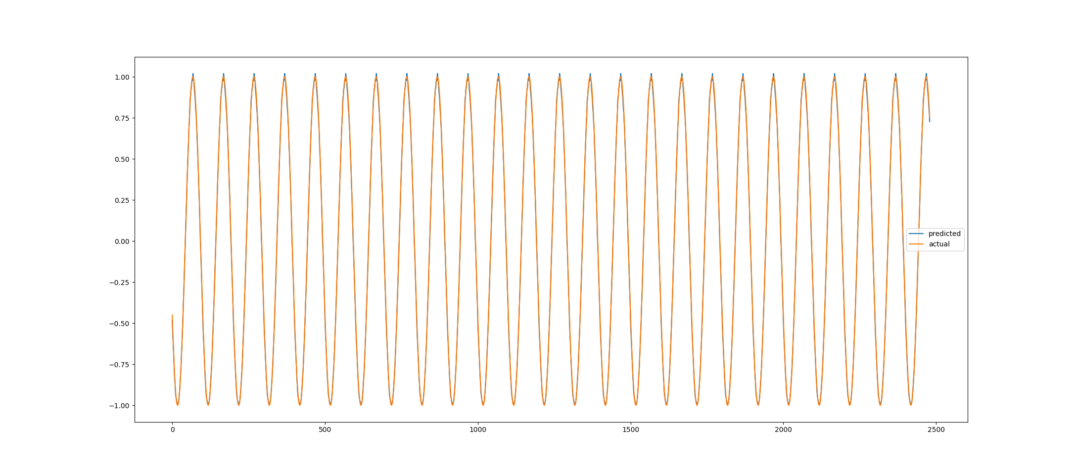
This looks pretty promising… but what happens if we attempt to train a network on the humidity data from the IoT sensors?

The Real Data

The first step in training and LSTM network to the humidity data captured by the IoT sensors is getting access to the data. The data from the IoT sensors gets saved in a web app called BeeBotte.

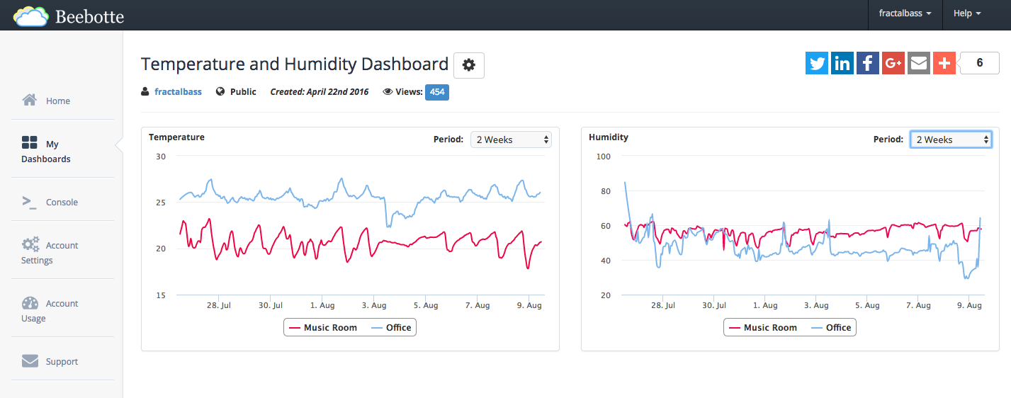
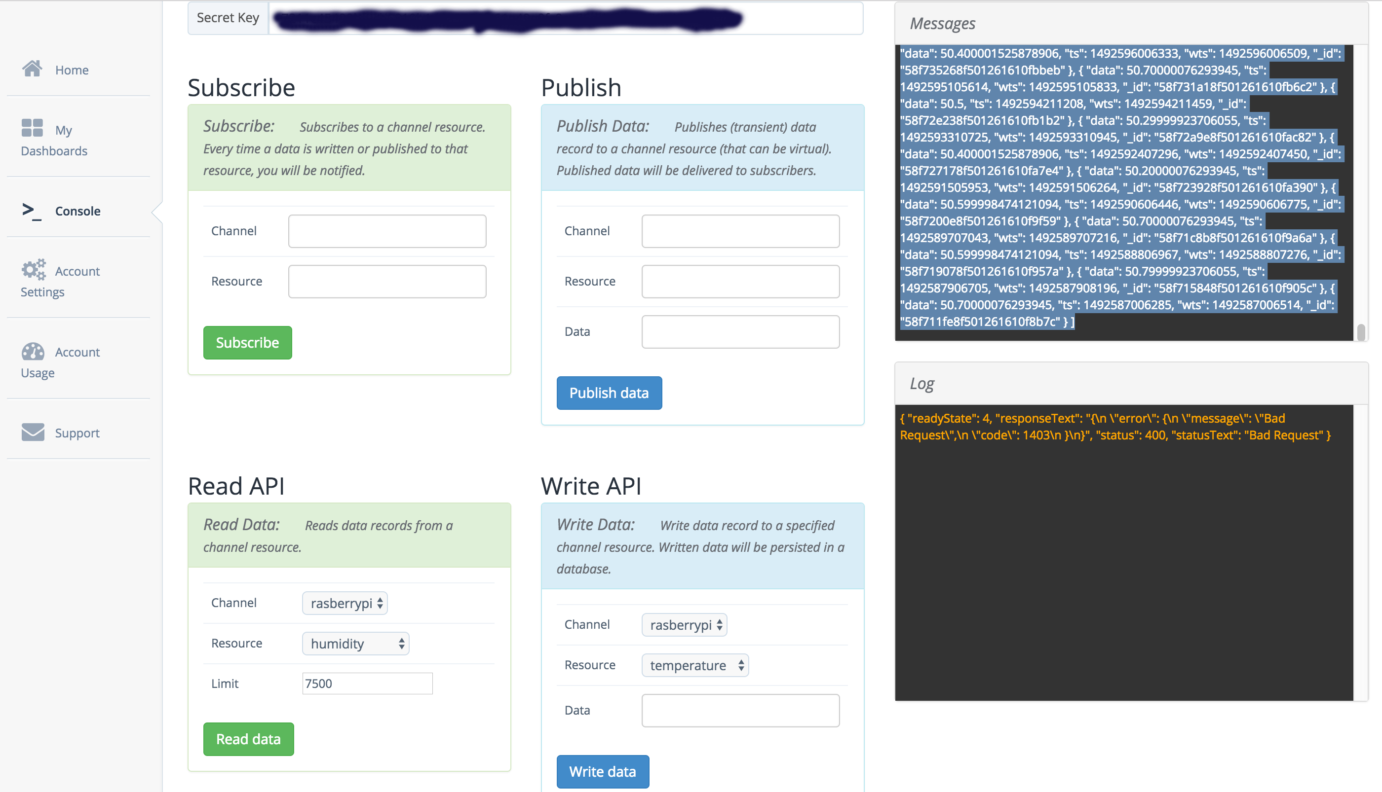
Before anything can be done with the data, it needs to be extracted from Beebotte. At first glance, it may appear that getting the data could be as simple as looking at the backend query that powers the BeeBotte dashboard (shown above). The BeeBotte dashboard makes a call to the BeeBotte API when it displays the data on their dashboard pages. Chrome developer tools can be used to view this raw data. (See the Hall of Justice blog post on using this approach.) Unfortunately, that technique won’t work in this case because Beebotte reduces the number of data points when the backend query attempts to pull data from too far in the past or too wide a data window. Fortunately, BeeBotte does provide a “console” in their website where a more complete dataset can be obtained.

Data Format

In the case of BeeBotte, their backend API and console return data in a JSON (Java Script Object Notation) format. You can see this if you make a call to their API.

[{
	"_id": "5978d52b0e4d72e331438b05",
	"data": 86.30000305175781,
	"ts": 1501091115636,
	"wts": 1501091115850
}, {
	"_id": "5978ce3f0e4d72e331438174",
	"data": 83.0999984741211,
	"ts": 1501089343454,
	"wts": 1501089343668
}, ...

While this is handy for use with dashboards and front-end web site development, it is not the best format to use with Python based tools like Pandas, Numpy or Keras. Also, the data provided in the JSON file is listed from the most recent measurement first. In order to get the data to work as an input to an RNN, it needs to be converted into a format like this:

69.4000015258789
69.4000015258789
66.4000015258789
64.30000305175781
62.20000076293945
61.900001525878906
61.0
60.099998474121094
60.0
57.900001525878906
57.29999923706055
57.20000076293945
...

The above sample was taken from a file generated by the class file_helper.py. This file, and the complete code for this blog post can be found in the GIT repository for this project.

Real World Results

When running the real world data through our RNN (after we scale the data so that it fits between -1 and 1) we get the following graph:

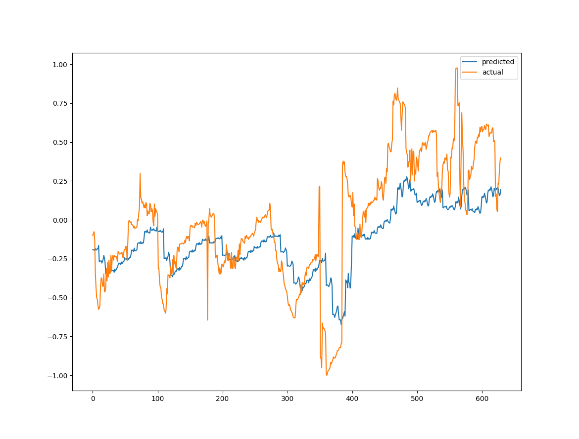
It does appear that the network is getting the general sense of the data. One thing to note on this graph is that I am actually displaying sets of outputs of 10 values each. The lines on the graph below may help visualize what is happening. The curves between the vertical blue bars are the actual data (yellow curve) and the LSTMs guess at the data (blue curve). In a number of other posts on this subject, the LSTM networks are always trained to output only a single value. In my implementation the next 10 points in the LSTMs guess are based on the input of the preceding 40 real values. This means that the network is constantly referring back to the “Real Data” when making estimates. Jakob Aungiers post on time series forcasting goes into some analysis as to what happens if you continue to base the LSTMs guesses on it’s own outputs.

The following figure shows how the sets of 10 output points are broken up in the diagram.

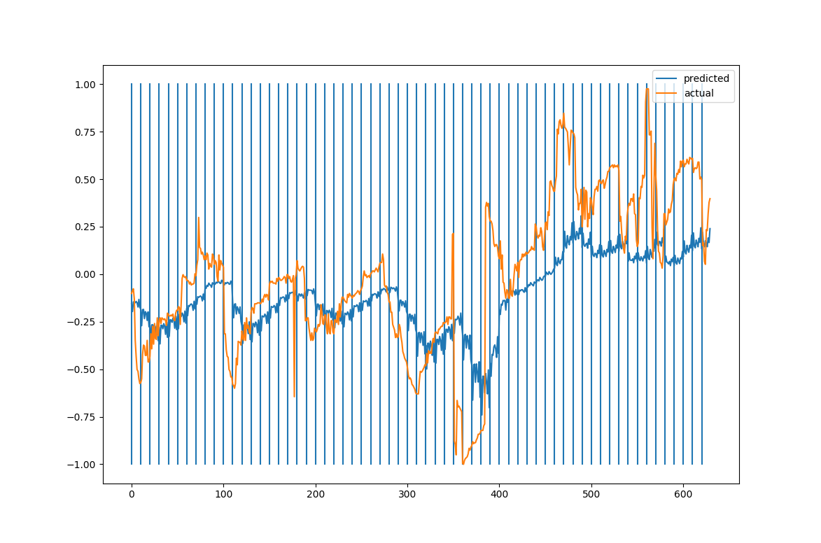
The blue curve above are outputs from a network that was only trained on a single epoch of the data. We can do a bit better if we increase the number of training epochs to 100. (I have removed the blue lines to make the graph easier to read.)

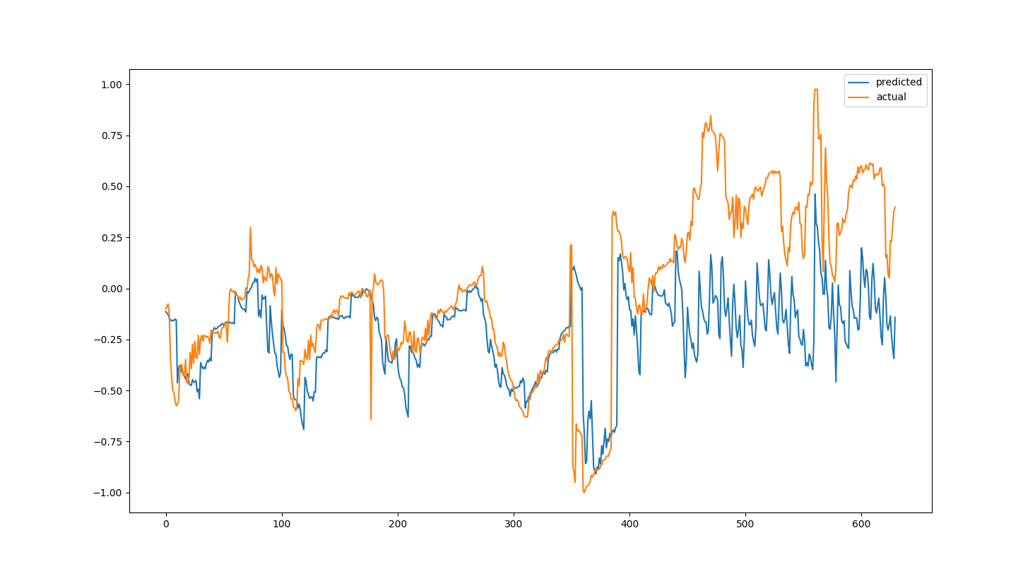
This is actually starting to look better. One potential use of the trained network could then be to set off some kind of alert when the predicted and actual value of the network starts to fall outside some range.

Don’t Look For Logic Where There Is None

This is all interesting stuff, but I want to put in a word of caution here. I have a saying:

Don’t look for logic where there is none.

While the saying was meant to be used when organizations or people make crazy decisions, I think it may actually apply in this case. The underlying data for the humidity in my house is a function of an infinite number of variables. They include, but are not limited to, the time of year, the temperature in the house the humidity outside of the house, if anybody is taking a shower, or cooking pasta, etc. etc.

I think that it is sometimes tempting to think that we can use neural networks to predict behavior in situations where there are nearly infinite variables. And, if we cannot get our network to learn patterns we may be tempted to either crank up the training epochs, or the number of the nodes in the network in order to get our learning curves to do what we would want them to do.

In the case of this project, that is exactly what I did. There was, however, a simpler way.

This whole episode started when the humidity in my house was so high that the paint caused problems with the knockdown. That is easily detected by just comparing the actual humidity to some fixed value, say 75%. I don’t mean to bash neural networks, but I do think it is worth considering using the simplest possible approach to problems rather than creating elaborate solutions.

On second thought…

If I looked for the simplest solution to problems, my blog posts would be pretty boring. (And, to the relief of many, probably much shorter.)

Conclusion

In this blog post we have looked at using Long Short Term Memory (LSTM) networks to predict time series data. LSTMs are a type of RNN that are better at overcoming the problem of “Vanishing Gradients”, which many RNNs are susceptible to.

The data in this blog post came from an external source and was in JSON format. We were able to convert that format to a much handier .CSV format.

We also looked at how testing can be incorporated into a data-science model, and discussed why testing should be considered whenever dealing with any kind of machine learning solution.

I hope you have enjoyed this post. It was probably the most time-consuming and confusing data science blog post I have taken on to date. I must say, seeing the thing actually work is pretty gratifying.

If you have any questions or comments about the post, please feel free to email me at the link below.

Stay tuned for more interesting topics in data science and machine learning!