Bayesian Inference Part 2: Data Science, Its Yuge!
Bayesian Inference Part 2: Data Science, It’s Yuge!

Introduction
This post will expand on some of the topics discussed in the last post… without the cat. There has been considerable discussion about the tweeting habits of President Trump. Trump has tweeted over 32,000 times since 2009. These tweets provide an excellent source of raw material for Bayesian techniques and analysis.
A bit of a disclaimer…
The goal of this post is to use Bayesian Inference and the Python Natural Language Toolkit to explore the nature of President Trump’s tweets (dating back to 2009). I am not trying to make a political statement, but rather present some data science techniques that can be applied to this data set. There may be a number of ways to interpret these results and “spin” them. I will leave any political assessments and conclusions to the reader.
Let’s begin by expanding on the discussion in the last post about Bayes’ Theorem and introduce the concept of Bayesian Inference.
Bayesian Inference
The equation that we get from Bayes’ Theorem looks like this:
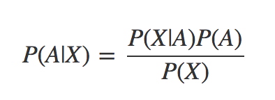
In this formula we refer to P(A|B) as the posterior probability and P(A) as the prior probability. As new information comes in about our experiment, we have the opportunity to iteratively apply Bayes’ Theorem by taking our last computed posterior probability e.g. P(A|B) and use it as a prior probability P(A) and compute a new posterior.
A great explanation of Bayesian Inference can be found in the following python notebook: http://nbviewer.jupyter.org/github/psinger/notebooks/blob/master/bayesian_inference.ipynb
What does this have to do with @realDonaldTrump, or vice versa?
As I mentioned in the introduction, President Trump is a great source for raw twitter data. His 32000+ tweets going back to 2009 provide a rather large data set for trying out some Bayesian Inference techniques. The first challenge in dealing with those tweets, is how to get ahold of them, however…
Obtaining the data
The repo https://github.com/mkearney/trumptweets has instructions for how to download all of the Trump tweets using R. I particularly enjoyed this part…
> ## run function to download Trump's twitter archive
> djt <- trumptweets()
    Downloading 31157 tweets...
    You're halfway there...
    Huzzah!!!
Using the above program, we can download the tweets and put them into a .CSV file and then switch back to python for the rest of our analytic tasks. In addition to just analyzing the frequency of President Trump’s tweets, I also have some interest in seeing how these tweets have changed tone over time.
We will start with analyzing President Trump’s number of tweets per day, and then look more closely at the sentiment of the tweets.
Analyzing the Tweet Frequency
First, we need to summarize the raw tweet data into a file that contains the number of tweets per day. Once we have the summarized data, we will save the results as an intermediate .CSV file for use in our analysis. (Be sure to check out the git repo for the latest version of the code associated with this post.)
#--------------------------------------------------------------
#  By Miles R. Porter
#  Painted Harmony Group, Inc
#  June 28, 2017
#  Please See LICENSE.txt
#--------------------------------------------------------------

import pandas as pd
import matplotlib
from pylab import *
import TrumpTweetUtilities

class TrumpCountDailySummarizer:

    def run(self):
        dt = pd.read_csv("./data/realdonaldtrump-fullarchive.csv")
        util = TrumpTweetUtilities.TrumpTweetUtilities()
        counts_df = util.count_rows_group_by_date(dt,"created_at")
        print(counts_df)
        counts_df.plot(kind="line")
        counts_df.to_csv("./data/trump_daily_counts.csv")
        plt.show(block=True)

tfa = TrumpCountDailySummarizer()
tfa.run()
You will note that the above program uses a module called TrumpTweeetUtilities. This module includes the logic for summarizing the tweets, and creating a dataframe with the counts by day. The module was test driven based, and you can check out the tests and code in the git repo mentioned above. I am not going to include the code here. (;tldr? You’re welcome.)
The graph of Trump’s tweets by day looks like this:
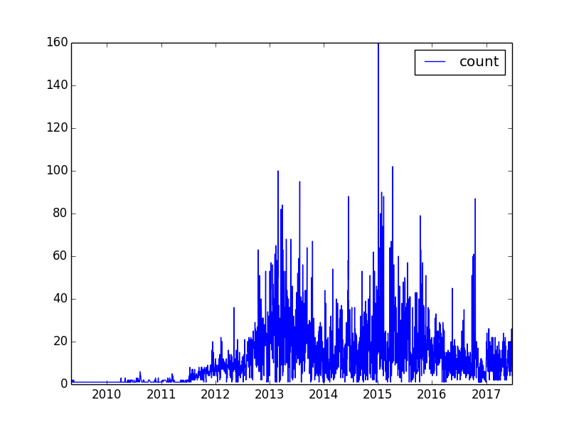
You may notice a huge spike in the data. That happened on January 5th, 2015. That was the date of an episode of “Celebrity Apprentice” titled, “Episode 2: “Nobody Out Thinks Donald Trump”…
This is going to be a special season - truly great characters and cast. You will soon see!
Trump (or somebody) tweeted throughout the show… 160 times. (Note that many of those were re-tweets.)
Analyzing the Frequency of Trump Tweets
Check out the second example in Davidson-Pilon’s Probabilistic Programming book chapter 1 python notebook. In the second example, Pilson uses Bayesian techniques to analyze his own tweeting habits over time. I borrowed heavily from this code, and modified it to work with the Trump tweet data.
The Poisson Distribution
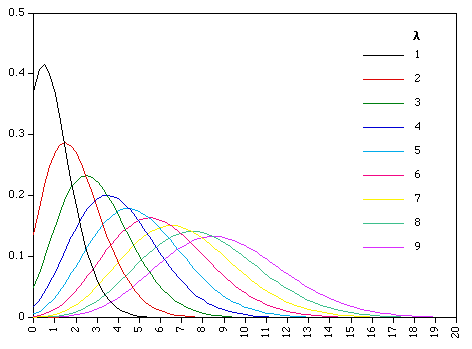
The technique used in “Probabilistic Programming and Bayesian Methods” by Cam Davidson-Pilon mentioned above uses Bayesian inference to split the time domain into two chunks. The first chunk (before time “tau”) and the second chunk (after time “tau”) are each associated with a probability distribution. These distributions are Poisson distributions and they each have their own lambda values. (Lambda is the parameter used in defining a Poisson distribution. For more info, check out this link on the Poisson Distribution.
Using Bayesian Techniques
Going back to the focus of this post, let’s restate what we are trying to investigate. On any given day there was a likely number of tweets that President Trump might make on that day.
- What was President Trumps earlier expected number of tweets per day?
- What was President Trumps later expected number of tweets per day?
- At what date did president trump start tweeting more or less?
To approach this in a Bayesian way, we want to focus on probability distributions that are associated with each of the above statements.
To kick things off, for each of the implied distributions above, we start with a given value for lambda that we make up. That is our Bayesian “prior”. It turns out that the value that we pick for the prior doesn’t really matter that much. Once we have our prior, we iteratively compute a posterior probability, and then use it as the next prior. We continue to follow this process using a technique called Markov Chain Monte Carlo to help us eventually create probability distributions for lambda 1, lambda 2 and tau that fit our observed data. The heavy lifting in all of this is done by a python framework called PyMC3. You can also refer to Pilon’s book for more information about PyMC3.
(It was time for a graphic to break things up. Again, you’re welcome.)
The PyMC3 toolkit provides tools for implementing Bayesian techniques in python.
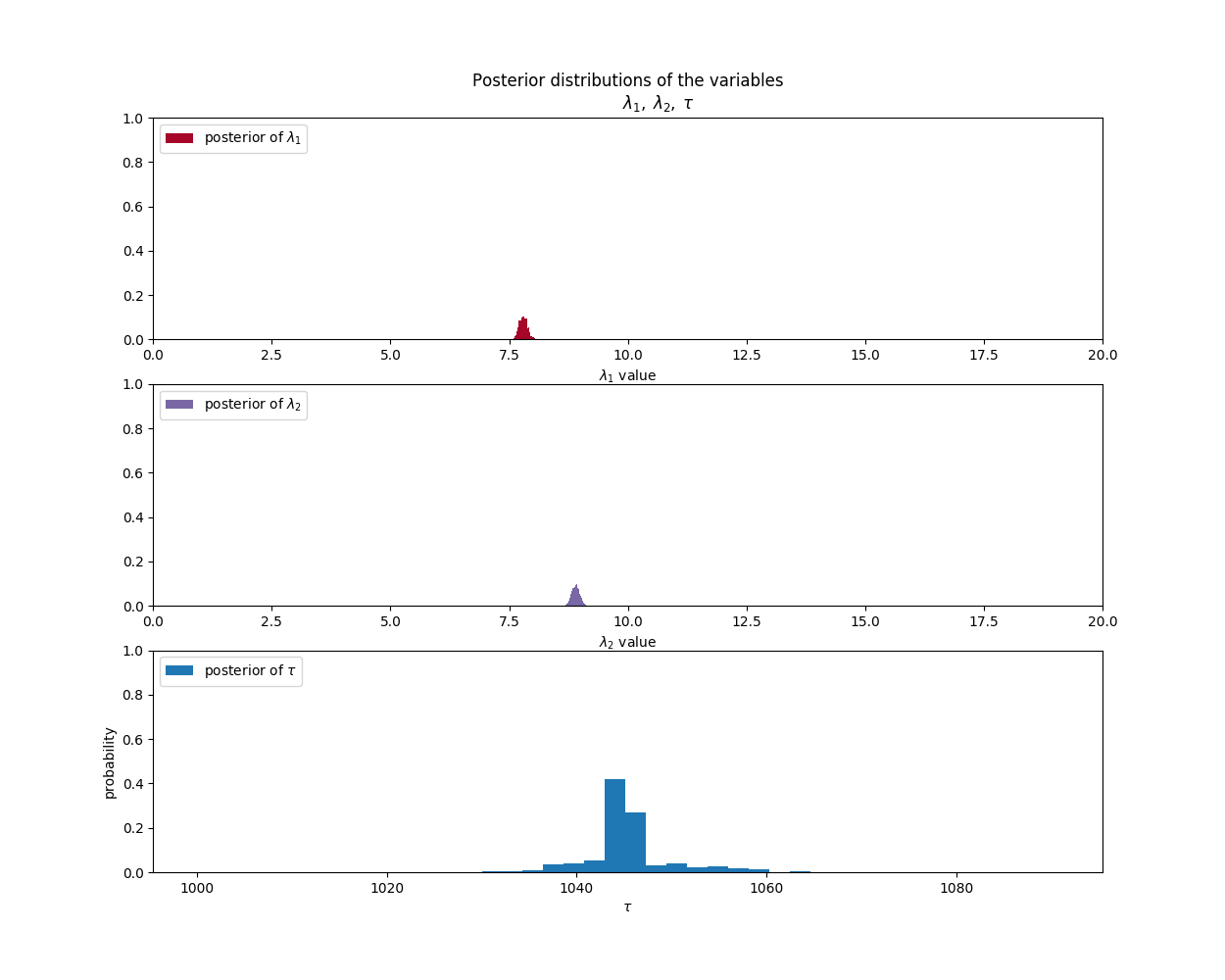
When we run the program, we come up with a final result that looks like this:
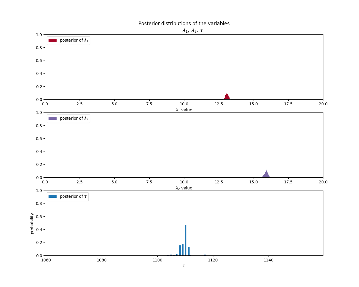
Based on that information, and the data the we have for the number of tweets per day, we can generate the following graph that shows the expected number of tweets per day based on the two distributions that are separated by the tau value.
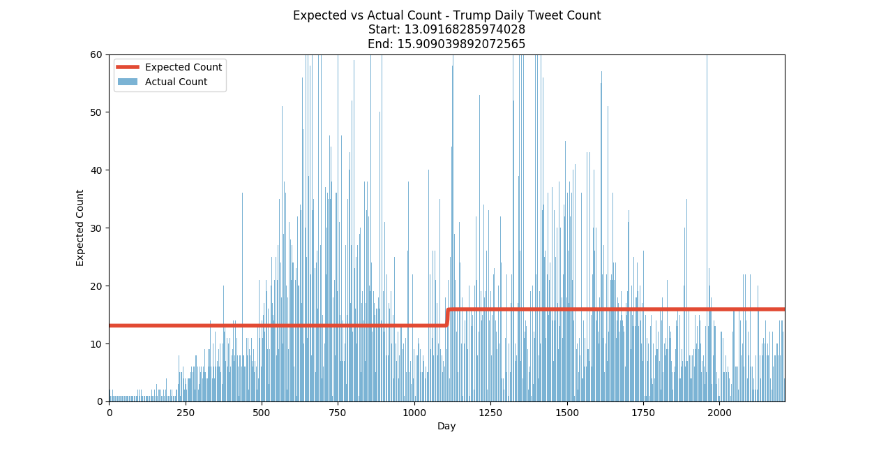
From this data, it would appear that President Trump’s tweeting habits changed around day 1100. If we go back to our summary data we can see that that day corresponds to June 29th, 2014.
What was special about that day? On day June 29, 2014, Donald Trump tweeted this…
Always remember, I was the one who got Obama to release his birth certificate, or whatever that was! Hilary couldn’t, McCain couldn’t. @realdonaldtrump 12:42 PM - 29 Jun 2014
Before that date, our probability distributions indicated that trump would most likely tweet around 13 times per day. After that date, he was most likely to tweet around 16 times per day. That may not sound like much, but keep in mind that is an average over more than 1000 days.
Now, lets repeat this experiment, but look at the sentiment of Trump’s tweet by day rather than just the total count.
Analyzing the tweet Sentiment
Now that we have a methodology to follow, lets see what happens if we apply the same technique to the positive and negative sentiment of President Trump’s tweets.
In order to assess the sentiment (positive or negative) of the tweets, we could go through each of the 32000 and manually classify them as either positive or negative; which might just drive us crazy. Another, less painful approach, could be to use the Python Natural Language Tool Kit, or NLTK as it is commonly referred to. In the git repo associated with this blog post there is a python class and test that I created to encapsulate using NLTK to assess the positive or negative sentiment of a tweet (or any string, really). The NLTK code uses Bayesian techniques to train a classifier based on a set of known data, or corpus.
There are two steps we need to go through before we start analyzing the data. The first step that we walked through above is to go through the original data and indicate if each tweet was either positive or negative. The second part is to roll up the counts for each day and save it to a .csv file like this:
created_at,count,neg,pos
2009-05-04,1,0.0,1.0
2009-05-05,1,0.0,1.0
2009-05-08,2,2.0,0.0
2009-05-12,2,0.0,2.0
2009-05-13,1,0.0,1.0
2009-05-14,1,0.0,1.0
2009-05-15,1,1.0,0.0
...
One of the most difficult parts of putting together this blog post was getting the sentiment analysis summaries in working shape. Python pandas has some pretty rich features, but it is still a pretty young release. As a result, there are a number of aspects to the module that don’t behave consistently. One of those areas is reading and writing .CSV files… particularly large .CSV files. The code associated with this post involved reading and summarizing (groupby in pandas terms) dataframes. To get that to work correctly, I needed to get sort of fancy with how I rolled up the positive and negative sentiment counts by day. This code shows what I had to do to get it to work…
    def sum_columns_in_grouped_rows_by_date(self, dataframe, date_col):
        dataframe["created_at"] = dataframe["created_at"].apply(lambda x: self.tryConvert(x))
        pos_counts = dataframe.groupby(dataframe[date_col]).agg({'pos':['sum','count']})
        neg_counts = dataframe.groupby(dataframe[date_col]).agg({'neg':['sum','count']})
        d = {"count": pos_counts["pos"]["count"].values,
             "pos": pos_counts["pos"]["sum"].values,
             "neg": neg_counts["neg"]["sum"].values}
        newdf = pd.DataFrame(d, index=pos_counts.index)
        return newdf

    def tryConvert(self, x):
        duh = None
        if isinstance(x, datetime.datetime):
            duh = x.date()
        else:
            try:
                duh = dateparser.parse(x).date()
            except:
                print("Failed to parse {0} ".format(x))
        return duh
Be sure to refer to the repository and the tests and code there for more info. Again… You’re welcome. :)
Finally the Results!
Here is a graph associated with the Bayesian analysis of the positive and negative sentiment for President Trump’s tweets by day.
Again, you can check out the code in the repo if you like. I will just cut to the graphs because this rather long blog post is getting even longer.
Positive Sentiment Parameter Analysis:
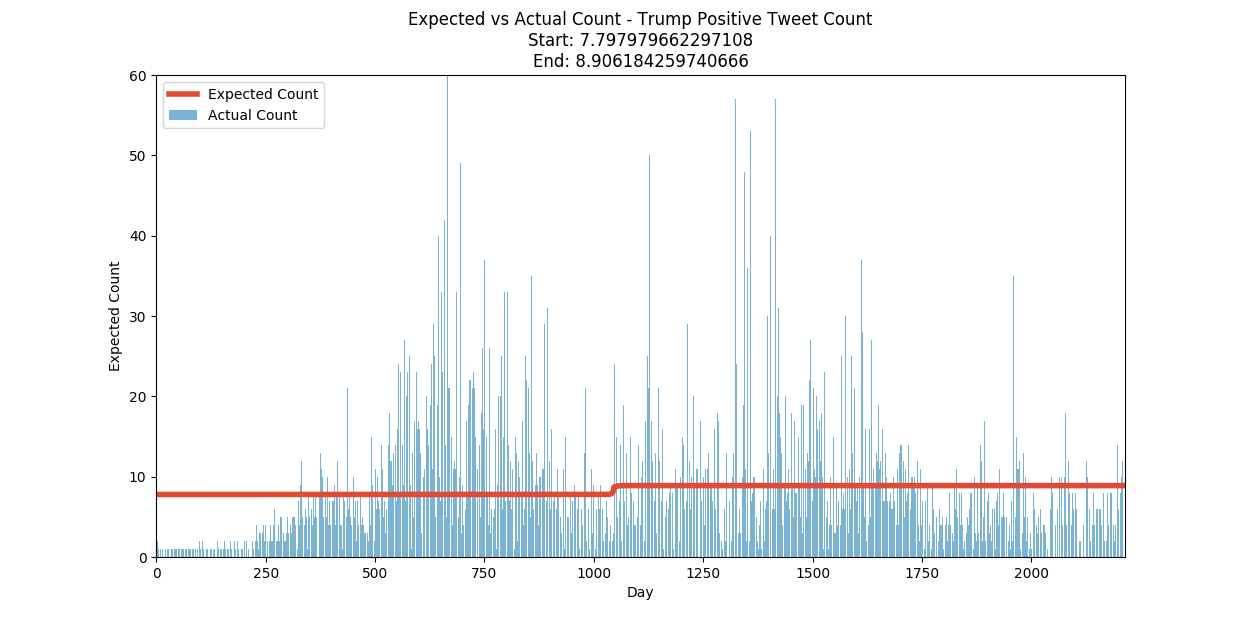
Positive Sentiment Summary:
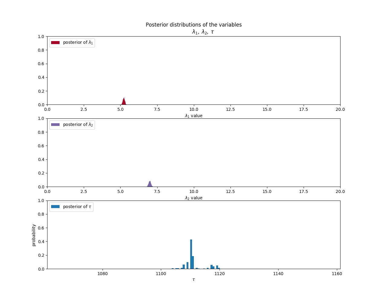
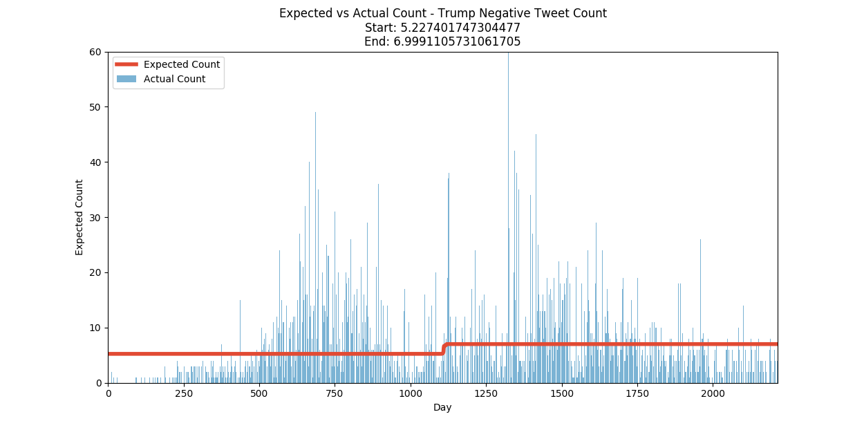
Negative Sentiment Parameter Analysis:
Negative Sentiment Summary:
Conclusion
Here are the results summarized in a single table…
| Probability Distribution | Initial Average | Cutover Date | Final Average |
|---|---|---|---|
| Total Tweet Count | 13 | Jan 5, 2015 | 16 |
| Positive Tweets/Day | 8 | March 20, 2014 | 9 |
| Negative Tweets/Day | 5 | June 3, 2014 | 7 |
The resulting probability distributions suggest that President Trump’s tweeting has increased, and that his tweets (as determined by the Python NLTK) are more likely to be positive than negative. It is interesting to note that the NLTK assessment thinks that Trump’s tweets are generally more positive than negative. However, the increase in the negatively assessed tweets have increased faster than the positive ones.
What does all this mean? That is for the political pundits to decide.
One thing is for sure, however. Mathematically, this assessment is not fake news.
I hope you have enjoyed this exploration into Bayesian Inference. Check back soon for more interesting topics in data science, and be sure to check out the resources below.
Have a great (and safe) 4th of July!
