LLMs Are Random Variables, Not Functions
Functions, Random Variables, and Why LLMs Are Not Deterministic Systems
In the United States, by around 8th grade (ages 13–14), students are introduced to the concept of a function. This idea becomes foundational across nearly all of mathematics, including algebra, trigonometry, Euclidean geometry, calculus, differential equations, linear algebra, and abstract algebra.
A standard definition of a function is:
A function is a relation between two sets that assigns each element of the first set to exactly one element of the second set.
More formally, if:
\[f : A \rightarrow B\]then for every:
\[x \in A\]there exists exactly one:
\[y \in B\]such that:
\[f(x) = y\]This “exactly one output per input” property is the key structural constraint that defines a function.
A Critical Asymmetry
It is important to emphasize a subtle but critical asymmetry:
- Multiple inputs may map to the same output (many-to-one is allowed)
- A single input may not map to multiple outputs (one-to-many is not allowed)
So it is perfectly valid that:
\[f(x_1) = y\]and
\[f(x_2) = y\]with
\[x_1 \neq x_2\]However, the following is not valid for a function:
\[f(x) = y_1\]and
\[f(x) = y_2\]with
\[y_1 \neq y_2\]This deterministic mapping structure is what makes functions so powerful. It forms the foundation for derivatives, integrals, transformations, and essentially all of continuous mathematics.
Random Variables and Probability
In probability theory, we introduce a different kind of object: the random variable.
A random variable is often defined as a function:
\[X : \Omega \rightarrow \mathbb{R}\]In this sense, a random variable is still technically a function.
The key difference is that we do not typically focus on the deterministic mapping itself. Instead, we associate the variable with a probability distribution that governs which outcomes are likely.
Rather than asking:
\[X(\omega) = x\]we ask questions such as:
\[P(X = x)\]or
\[P(X \in S)\]for some set $S$.
In other words, probability theory shifts the focus from deterministic outputs to distributions over possible outputs.
Statistics then reverses the direction of inference: we observe samples and attempt to infer properties of the underlying distribution.
Why LLMs Behave Like Stochastic Systems
This distinction becomes especially important when thinking about modern generative AI systems such as Large Language Models (LLMs).
At a computational level, an LLM can be viewed as a function:
\[f_{\theta}(p) \rightarrow \text{distribution over tokens}\]where:
- $p$ is the prompt
- $\theta$ represents the learned model parameters
However, the key point is that the model does not directly produce a single fixed output.
Instead, it produces a probability distribution, and the final response is typically obtained by sampling from that distribution:
\[y \sim P_{\theta}(\cdot \mid p)\]This means that for the same input prompt $p$, multiple different outputs $y$ can be generated across different runs.
So while the underlying model parameters are deterministic, the output generation process is stochastic.
A Simple Experiment
Consider the prompt:
“Write a paragraph about how to pick your favorite color.”
Running this prompt multiple times will produce different—but still valid—responses.
Each response is typically:
- Coherent
- Relevant
- Grammatically correct
Yet the responses will not necessarily be identical.
This variability is not noise in the traditional sense. It is a direct consequence of sampling from a learned probability distribution over language.
A More Complicated Experiment
The following plot shows how responses vary from LLM to LLM. This graph was generated by using the same prompt 100 times in each of the LLMs listed. The resulting language-related qualitative metrics were then calculated. Some models have a “temperature” parameter that can increase or decrease the amount of randomness or creativity in the LLM response. For this experiment, the temperature value was set to 0 for those models that have that parameter available. This encouraged the model to be as non-stochastic as possible when generating responses.
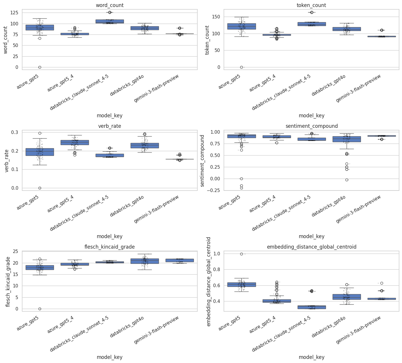
From the plot above, we can clearly see two things. First, across all of the LLMs, the response to the prompt was stochastic. Second, different models demonstrated different amounts of variance in the quantitative metrics of the text that was generated. (Note that this experiment was limited specifically to the English language.)
The prompt used for the experiment above was: “Write a concise paragraph explaining the significance of reproducibility in machine learning experiments.” The system prompt was: “You are a helpful assistant.”
The Value and Risk of Stochastic Generation
This stochasticity is central to both the power and the risk of LLMs.
Benefits
Stochastic generation enables:
- Creative variation
- Idea generation
- Exploration of alternative phrasings
- Discovery of alternative solutions
Risks
At the same time, it introduces:
- Non-zero probability of incorrect information
- Inconsistency across runs
- Difficulty in guaranteeing correctness without external verification
Importantly, these risks do not disappear with increased scale or capability.
They are structural properties of the sampling process itself.
Implications for Deployment
In practice, this means LLMs should not be treated as deterministic, truth-preserving systems.
They are better understood as probabilistic generators that require:
- Validation layers
- External grounding (retrieval systems, tools, databases, APIs)
- Testing across distributions of inputs
- Monitoring for failure modes over time
This is similar in spirit to how humans are evaluated in safety-critical roles.
We do not assume correctness from a single response or test. Instead, we rely on:
- Repeated evaluation
- Certification
- Ongoing oversight
- Performance monitoring
Closing Thought
LLMs are not simply “right or wrong” machines.
They are systems that generate outputs according to learned probability distributions.
That makes them powerful.
But it also means their outputs should be interpreted as:
Useful suggestions drawn from a distribution, not guaranteed facts.